Population dynamics of surface-mediated autocatalytic processes
Pith reviewed 2026-06-27 05:19 UTC · model grok-4.3
The pith
Particles diffusing toward surfaces that either kill or replicate them have their full population statistics captured by a generating function whose long-time behavior falls into one of three regimes.
A machine-rendered reading of the paper's core claim, the machinery that carries it, and where it could break.
Core claim
We provide a systematic analysis of the generating function of the population size. We also deduce its distribution, mean, variance and higher-order moments. For this purpose, we employ several equivalent descriptions of these quantities in terms of nonlinear integral equations and partial differential equations with nonlinear boundary conditions. We inspect the long-time behavior of the population dynamics in three regimes when the mean population size vanishes, reaches a steady-state level, or grows exponentially.
What carries the argument
The probability generating function of the population size, expressed through nonlinear integral equations or PDEs with nonlinear boundary conditions that encode the competing surface kill and replicate rates.
If this is right
- Exact expressions for the mean, variance, and all higher moments of the population follow directly from the generating function.
- The long-time mean population size is confined to one of three behaviors: decay to zero, approach to a positive constant, or exponential growth.
- The specific regime is selected by the relative magnitudes of the diffusion constant and the surface kill and replicate rates.
- Numerical inversion of the integral equations and direct Monte Carlo sampling both reproduce the analytic moments and regime boundaries.
Where Pith is reading between the lines
- The same generating-function approach could be applied to time-varying surface rates or to surfaces whose geometry changes with the population itself.
- The three regimes supply a parameter-free way to classify outcomes in any diffusion-limited system whose reactions are confined to fixed boundaries.
- Knowledge of the full distribution rather than only the mean would allow quantitative estimates of the probability of extreme population excursions.
Load-bearing premise
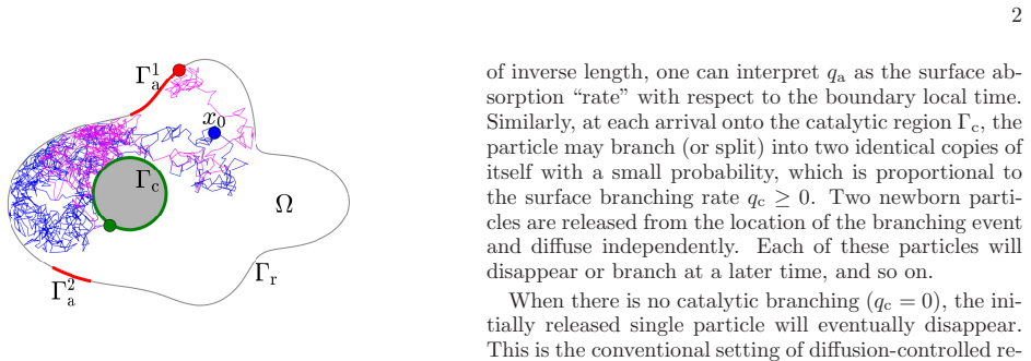
The model assumes particles undergo standard diffusion and that kill and replicate events occur only at fixed, localized surface regions.
What would settle it
A Monte Carlo simulation or laboratory experiment in which the long-time mean population grows neither to zero, nor to a constant, nor exponentially would falsify the claimed classification of regimes.
Figures
read the original abstract
We investigate the population dynamics of surface-mediated autocatalytic processes, in which particles diffuse in a complex environment towards surface regions where they can be either killed or replicated. These opposite mechanisms compete with each other and lead to a sophisticated stochastic evolution of the population size. We provide a systematic analysis of the generating function of the population size. We also deduce its distribution, mean, variance and higher-order moments. For this purpose, we employ several equivalent descriptions of these quantities in terms of nonlinear integral equations and partial differential equations with nonlinear boundary conditions. We inspect the long-time behavior of the population dynamics in three regimes when the mean population size vanishes, reaches a steady-state level, or grows exponentially. A numerical solution of the underlying integral equations and independent Monte Carlo simulations support our theoretical predictions.
Editorial analysis
A structured set of objections, weighed in public.
Referee Report
Summary. The manuscript analyzes the stochastic population dynamics of particles diffusing in a complex environment and undergoing competing kill/replicate reactions localized at fixed surface regions. It derives the probability generating function via equivalent nonlinear integral equations and PDEs with nonlinear boundary conditions, extracts the full distribution together with mean, variance and higher moments, and classifies the long-time asymptotics of the mean population size into three regimes (vanishing, steady-state, exponential growth). Numerical solution of the integral equations and independent Monte Carlo simulations are presented in support of the analytic predictions.
Significance. If the derivations hold, the work supplies a systematic stochastic-process treatment of surface-localized birth-death competition coupled to diffusion, including explicit moment expressions and regime classification. The equivalence of integral-equation and PDE formulations, together with the numerical/Monte-Carlo cross-validation, constitutes a concrete technical contribution to the modeling of autocatalytic processes in heterogeneous media.
minor comments (2)
- The abstract and introduction refer to 'complex environment' without a precise geometric definition; a short paragraph or figure in §2 clarifying the domain and surface placement would improve reproducibility.
- The long-time regime classification is stated in terms of the mean population size; it would be useful to indicate explicitly in the text (near Eq. (X) or the regime table) whether the higher moments follow the same asymptotic classification or exhibit different scaling.
Simulated Author's Rebuttal
We thank the referee for the positive summary of our work on the stochastic population dynamics of surface-mediated autocatalytic processes and for the favorable significance assessment. The recommendation of minor revision is noted. No specific major comments were provided in the report.
Circularity Check
No significant circularity detected
full rationale
The paper derives the probability generating function for population size via equivalent nonlinear integral equations and PDEs with nonlinear boundary conditions starting from the diffusion-reaction model assumptions. Moments and long-time regimes (vanishing, steady-state, exponential growth) follow directly from analysis of the mean and higher moments without any fitted parameters renamed as predictions or self-citation chains. Monte Carlo and numerical solutions serve as independent validation rather than inputs. All steps are self-contained standard stochastic process techniques with no reduction to the target results by construction.
Axiom & Free-Parameter Ledger
axioms (2)
- domain assumption Particles undergo standard Brownian diffusion in a complex environment
- domain assumption Kill and replicate mechanisms are localized to specific surface regions and compete
Reference graph
Works this paper leans on
-
[1]
However, this function must remain bounded between 0 and 1, so that such a growth is not possible
would imply an exponential growth of ¯Gs(t|x0). However, this function must remain bounded between 0 and 1, so that such a growth is not possible. Even though this equation re- mains valid, it is not suitable for the analysis of the su- percritical regime, and we switch to Eq. ( 18), which in- volves the decaying functions P +(x, t |x0) and S+(t|x0). This...
-
[2]
Is it possible to get a nonzero steady- state solution? Let us first assume that such a nontrivial solution exists and then inspect the conditions for its existence
that ¯Gs ≡ 0 is always a solution in the limit t → ∞ . Is it possible to get a nonzero steady- state solution? Let us first assume that such a nontrivial solution exists and then inspect the conditions for its existence. Replacing ¯Gs(t|x0) by its limit ¯Gs(∞| x0) in Eq. ( 18), we get in the leading order ¯Gs(∞| x0) = qc ∫ Γ c dx G+(x, x0) ( 2 ¯Gs(∞| x) − ...
-
[3]
Given that ¯G1(t|x0) ≡ 0 due to the probability distribution normalization, one might expect that ¯Gs(∞| x0) ≡ 0 for any s
does not also depend on s. Given that ¯G1(t|x0) ≡ 0 due to the probability distribution normalization, one might expect that ¯Gs(∞| x0) ≡ 0 for any s. We will argue below that this conclusion is valid in the subcritical and critical regimes. In turn, a strictly positive solution ¯Gs(∞| x0) > 0 does exist in the super- critical regime for s < 1, and this s...
-
[4]
as Gs(∞| x0) = π (x0) + qc ∫ Γ c dx G+(x, x0) [Gs(∞| x)]2, (49) where π (x0) = 1 − qc ∫ Γ c dx G+(x, x0). (50) The integral equation ( 49) has a simple probabilistic interpretation: in the steady-state regime, a particle started from x0 is either absorbed on Γ a with proba- bility π (x0), or branches at a point x ∈ Γ c, creating two identical independent ...
-
[5]
(58) Since both ¯Gs(∞| x0) and v0(x0) are nonnegative, this equality is only possible if qc/µ 0 > 1
by v0(x0) and integrate over Γ c that yields, due to the self-adjoint character of the operator A: ( 1 − qc µ 0 ) ∫ Γ c dx0 v0(x0) ¯Gs(∞| x0) = − qc µ 0 ∫ Γ c dx v0(x)[ ¯Gs(∞| x)]2. (58) Since both ¯Gs(∞| x0) and v0(x0) are nonnegative, this equality is only possible if qc/µ 0 > 1. In the marginal case, the left-hand side is zero, implying ¯Gs(∞| x) ≡ 0. ...
-
[6]
( 38): qk = − 1 k! lim s→ 0 ∂ k s gs (60) = δk, 1 + qcD C− 0 ∫ Γ c dx u− 0 (x) ∞∫ 0 dt′ eDt′λ − 0 Hk(t′|x), with Hk(t|x) given by Eq
immediately 12 implies the same asymptotic behavior, Qk(t|x0) ≃ qk u− 0 (x0) C− 0 e− Dtλ − 0 (t → ∞ ), (59) where the prefactor qk is obtained by differentiating the amplitude gs from Eq. ( 38): qk = − 1 k! lim s→ 0 ∂ k s gs (60) = δk, 1 + qcD C− 0 ∫ Γ c dx u− 0 (x) ∞∫ 0 dt′ eDt′λ − 0 Hk(t′|x), with Hk(t|x) given by Eq. ( 24). (ii) In the critical regime, ...
-
[7]
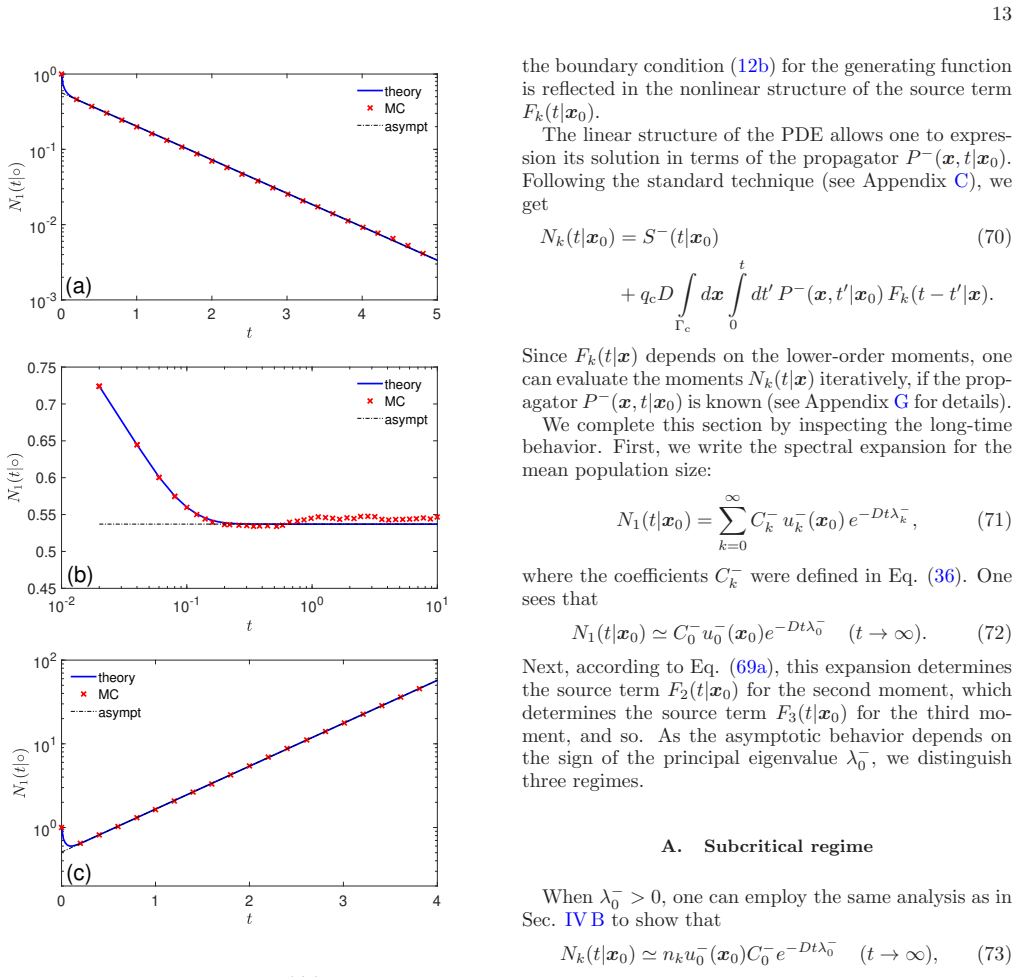
The linear structure of the PDE allows one to expres- sion its solution in terms of the propagator P − (x, t |x0)
is linear in Nk(t|x0), whereas the nonlinearity of the boundary condition ( 12b) for the generating function is reflected in the nonlinear structure of the source term Fk(t|x0). The linear structure of the PDE allows one to expres- sion its solution in terms of the propagator P − (x, t |x0). Following the standard technique (see Appendix C), we get Nk(t|x0...
-
[8]
in terms of products of lower-order moments, one can resort to the induction argument, i.e., one can assume that Eq. (
-
[9]
, k − 1 and then check it for k
holds for j = 1, 2, . . . , k − 1 and then check it for k. This assumption implies the long-time behavior Fk(t|x0) ≃ (u− 0 (x0)C− 0 )2e− 2Dtλ − 0 k− 1∑ j=1 (k j ) njnk− j, (74) so that the Laplace transform of Fk(t|x0) does not have a pole at p0 = − Dλ − 0 . As a consequence, the long-time asymptotic behavior of the right-hand side of Eq. (
-
[10]
( 73) by setting nk = 1 + qcD C− 0 ∫ Γ c dx u− 0 (x) ∞∫ 0 dt′ eDt′λ − 0 Fk(t′|x)
is Nk(t|x0) ≃ C− 0 u− 0 (x0)e− Dtλ − 0 + qcDu− 0 (x0)e− Dtλ − 0 ∫ Γ c dx u− 0 (x) ∞∫ 0 dt′eDt′λ − 0 Fk(t′|x), 14 that is reduced to Eq. ( 73) by setting nk = 1 + qcD C− 0 ∫ Γ c dx u− 0 (x) ∞∫ 0 dt′ eDt′λ − 0 Fk(t′|x). (75) As in Sec. IV B, the inconvenience of this representa- tion is that one needs to know Fk(t′|x) for all t′ > 0. If the long-time relati...
-
[11]
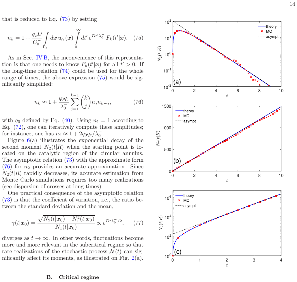
Since N2(t|R) rapidly decreases, its accurate estimation from Monte Carlo simulations requires too many realizations (see dispersion of crosses at long times)
with the approximate form (76) for n2 provides an accurate approximation. Since N2(t|R) rapidly decreases, its accurate estimation from Monte Carlo simulations requires too many realizations (see dispersion of crosses at long times). One practical consequence of the asymptotic relation (
-
[12]
is that the coefficient of variation, i.e., the ratio be- tween the standard deviation and the mean, γ(t|x0) = √ N2(t|x0) − N 2 1 (t|x0) N1(t|x0) ∝ eDtλ − 0 / 2, (77) diverges as t → ∞ . In other words, fluctuations become more and more relevant in the subcritical regime so that rare realizations of the stochastic process N (t) can sig- nificantly affect its m...
-
[13]
More explicitly, we have N2(t|x0) ≃ u− 0 (x0)C− 0 ( 1 + 2Dt qcq0 ) , (78) with exponentially decaying correction terms
yields t in the leading order. More explicitly, we have N2(t|x0) ≃ u− 0 (x0)C− 0 ( 1 + 2Dt qcq0 ) , (78) with exponentially decaying correction terms. In the Laplace domain, this behavior means that the product of two functions with a simple pole p0 = 0 yields a func- tion with a double pole p0 = 0. Repeating this procedure iteratively, one gets Nk(t|x0) ...
-
[14]
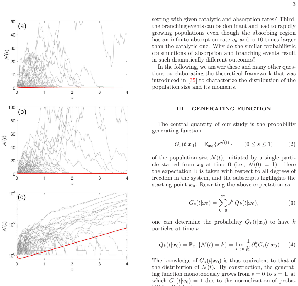
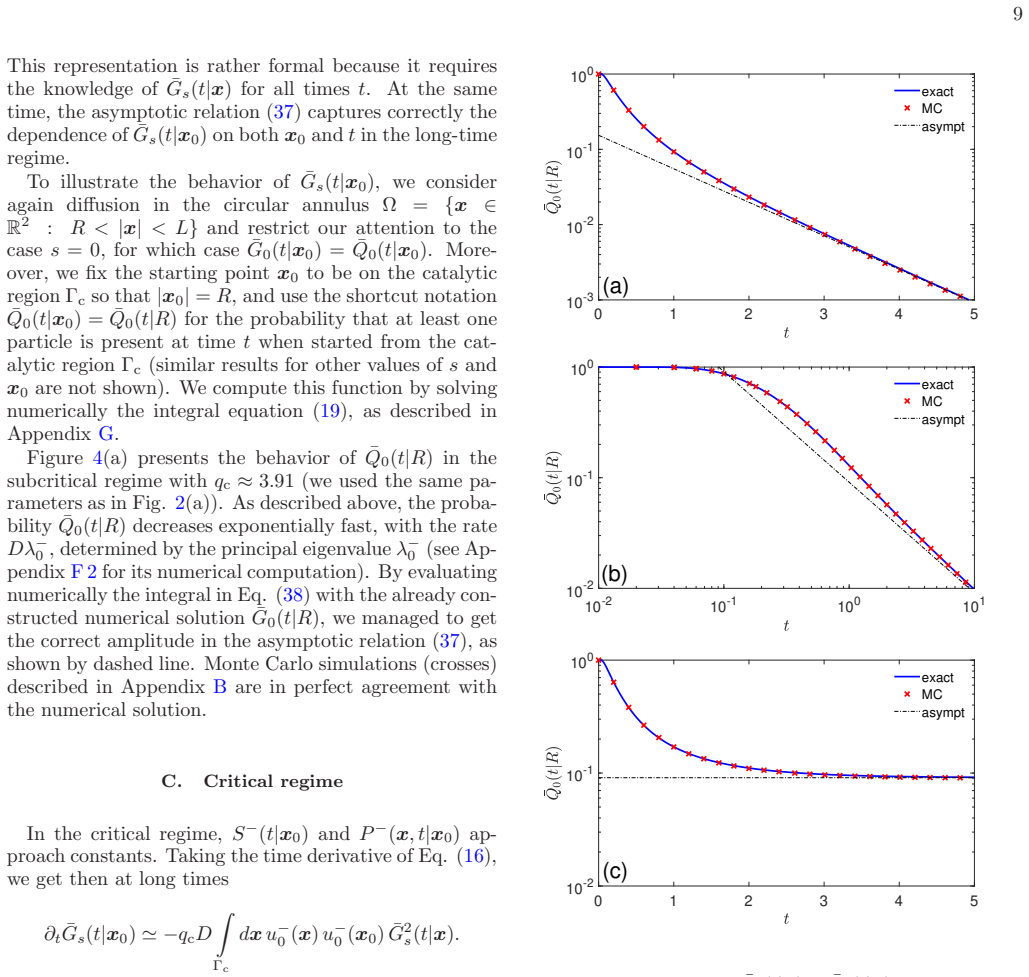
34); and (c) supercritical (qc = 1
91); (b) critical ( qc = qcrit c ≈ 4. 34); and (c) supercritical (qc = 1. 1 qcrit c ≈ 4. 78), with qcrit c = 1/ (R ln(L/R )). Solid blue line presents the exact result obtained via a numerical solu - tion of the integral equation ( 70) as described in Appendix G; crosses show the empirical mean of N 2(t) obtained over 10 6 random realizations (see Appendi...
-
[15]
implies Fk(t|x0) ∝ ekDt|λ − 0 | and this function determines the asymptotic behavior of Nk(t|x0). Using the Laplace transform and the above argument for the poles, we get the long-time behavior Nk(t|x0) ≃ qcDekDt|λ − 0 | ∫ Γ c dx (k− 1∑ j=1 (k j ) nj(x)nk− j(x) ) × ∞∫ 0 dt′e− kDt′|λ − 0 | P − (x, t ′|x0). (81) The dependence on the starting point x0 is th...
-
[16]
The time derivative of Eq
or ( 26), or by solving the initial-value problem ( 27) with k = 0. The time derivative of Eq. ( 22) yields an integral equation for the probability density: J0(t|x0) = Ja(t|x0) + 2qcD ∫ Γ c dx t∫ 0 dt′P +(x, t ′|x0) × Q0(t − t′|x)J0(t − t′|x), (87) 16 where Ja(t|x0) = qaD ∫ Γ a dx P +(x, t |x0) (88) is the flux of particles onto the absorbing boundary Γ a...
-
[17]
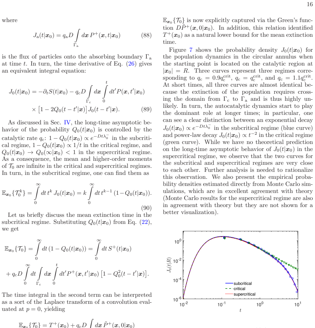
In addition, this relation identified T +(x0) as a natural lower bound for the mean extinction time
still depends on the probability Q0(t|x), the spatial dependence of the mean Ex0 {T0} is now explicitly captured via the Green’s func- tion D ˜P +(x, 0|x0). In addition, this relation identified T +(x0) as a natural lower bound for the mean extinction time. Figure 7 shows the probability density J0(t|x0) for the population dynamics in the circular annulus ...
-
[18]
paradoxical
1 qcrit c ≈ 4. 78, dotted red line), with qcrit c = 1 / (R ln(L/R )). The function J0(t|R) was obtained at short times by solv- ing numerically the integral equation ( 89); at longer times, J0(t|R) was calculated directly from a finite-difference ap- proximation of the derivative of Q0(t|R). Symbol present the empirical probability densities in the first two...
2024
-
[19]
Moreover, as the PDE problem ( E1) is linear, one can write its solution as N A 1 (t|x0) = ∫ A dx P − (x, t |x0)
for N1(t|x0) reveals the only difference in the initial condition. Moreover, as the PDE problem ( E1) is linear, one can write its solution as N A 1 (t|x0) = ∫ A dx P − (x, t |x0). (E2) As the mean population size in any subset A of the do- main can be obtained by integrating the propagator over A, P − (x, t |x0)dx can be interpreted as the mean popu- lati...
-
[20]
Principal Steklov eigenmode As discussed in the main text, the principal eigenvalue µ 0 of the Steklov problem (
-
[21]
As the principal eigenfunction is rotationally invariant, one can search it as v0(x) = A(ln(|x|/R ) + B), with two unknown constants A and B
determines the condition for the critical regime. As the principal eigenfunction is rotationally invariant, one can search it as v0(x) = A(ln(|x|/R ) + B), with two unknown constants A and B. Two boundary conditions fix the eigenvalue, µ 0 = 1 R[1/ (qaL) + ln(L/R )] , (F1) and the constant B so that v0(x) = A ( ln(L/ |x|) + 1 qaL ) . (F2) 22 The remaining ...
-
[22]
Principal Laplacian eigenmode In this section, we summarize the standard formulas to compute the principal eigenvalue λ − 0 and the associated eigenfunction u− 0 (x) by solving Eqs. ( 28). While this computation can be easily adjusted to get other Lapla- cian eigenmodes [ 58–60], we focus on the principal eigen- mode that determines the long-time behavior...
-
[23]
(F8d) In the following, we treat separately three regimes
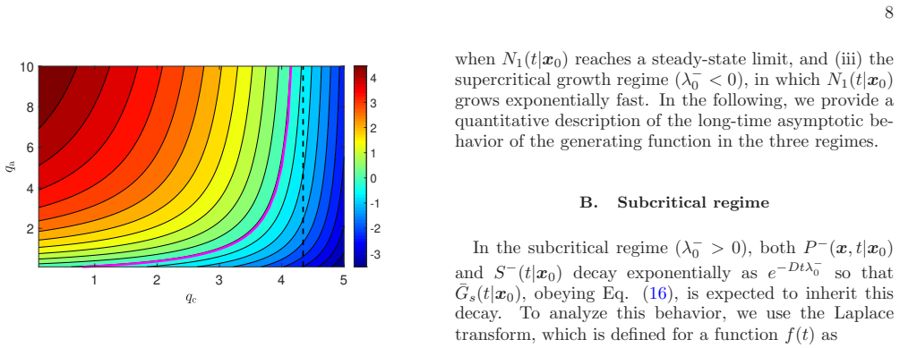
by replacing qc by − qc, and for the principal eigenpair {λ 0, u 0(x)} associated to qc = 0 and satisfying − ∆ uk = λ kuk in Ω , (F8a) ∂nuk = 0 on Γ c, (F8b) ∂nuk + qauk = 0 on Γ a, (F8c) ∂nuk = 0 on Γ r. (F8d) In the following, we treat separately three regimes. Subcritical regime In the subcritical regime ( qc < µ 0), the principal eigen- value λ − 0 is...
-
[24]
Integrating u− 0 (x) over Ω, we also get C− 0 = πA ( (L2 − R2)(1/ 2 + 1/ (qaL)) − R2 ln(L/R ) )
and ( 52) for the Laplacian and Steklov eigenmodes are identical, so that the principal Laplacian eigenfunc- tion u− 0 is actually proportional to the principal Steklov eigenfunction v0 (we recall that these eigenfunctions have different normalizations): u− 0 (x) = A ( ln(L/ |x|) + 1 qaL ) , (F16) where the normalization constant A is obtained from 1 = ∫ Ω...
-
[25]
To avoid technical details, we focus on the Laplace-transformed propagator, for which the computation is simpler: ˜P − (x, p |x0) = ∞∫ 0 dt e− pt P − (x, t |x0)
The propagator Since the Laplacian eigenmodes are known for the cir- cular annulus, the propagator P − (x, t |x0) can be found through the spectral expansion ( 31). To avoid technical details, we focus on the Laplace-transformed propagator, for which the computation is simpler: ˜P − (x, p |x0) = ∞∫ 0 dt e− pt P − (x, t |x0). (F25) Moreover, as our setting...
-
[26]
Mean population size For the circular annulus, an explicit computation of the mean population size N1(t|x0) is possible in the Laplace domain. For this purpose, it is sufficient to integrate the Laplace-transformed propagator ˜P − (x, p |x0) over Ω that yields ˜N1(p|r0) = 1 p ( 1 + qc vL(r0) − qa vR(r0) W ) , (F32) where vL(r0), vR(r0) and W are given by Eq...
-
[27]
Long-time limit of the generating function Since the annulus is rotationally invariant, the depen- dence of the generating function Gs(t|x0) on x0 is re- duced to the radial coordinate r0 = |x0|. As a conse- quence, the Green’s function G+(x, x0) in the integral equation ( 45) is averaged over the angular coordinate, yielding g(r0) = qc ∫ Γ c dx G+(x, x0)...
-
[28]
In turn, one has G1(t|x0) = 1 due to the normalization of probabilities in any regime. Appendix G: Numerical solution of integral equations In this Appendix, we present a numerical scheme for solving integral equations ( 25, 26) to determine the prob- abilities Qk(t|x0), as well as the generating function Gs(t|x0), in the case of the circular annulus with...
-
[29]
To see this point, we inspect the auxiliary function f (t) = ∫ Γ c dx0 ∫ Γ c dx P (x, t |x0) (G2) in the general setting
Short-time behavior of the kernel Let us first discuss the weak singularity of the kernel P (R, t ′|R). To see this point, we inspect the auxiliary function f (t) = ∫ Γ c dx0 ∫ Γ c dx P (x, t |x0) (G2) in the general setting. We assume that Γ a and Γ c are disconnected regions of the boundary (as in the case of the circular annulus). As a consequence, Γ a ...
-
[30]
These quantities can be found either in terms of spectral expan- sions over the Laplacian eigenfunctions, or via the inverse Laplace transform
Numerical computation of the kernel To proceed, we need to evaluate S(t|R) and p(t). These quantities can be found either in terms of spectral expan- sions over the Laplacian eigenfunctions, or via the inverse Laplace transform. In the Laplace domain, we can use Eq. ( F28) to get ˜P (R, p |R) and Eq. ( F32) to get ˜S(p|R), by setting qc = 0. We employ the...
-
[31]
( G6) as ¯Q0(nδ) ≈ S(nδ|R) + n∑ j=0 wj v((n − j)δ), (G10) where wj are suitable weights
Discretization Choosing a small timestep δ = t/n and equally spaced grid, we discretize Eq. ( G6) as ¯Q0(nδ) ≈ S(nδ|R) + n∑ j=0 wj v((n − j)δ), (G10) where wj are suitable weights. In a basic quadrature, we use piecewise-constant ap- proximations for functions p(t′) and v(t − t′) on each interval (δj, δ (j + 1)), so that tj+1∫ tj dt′ √ t′ p(t′) v(t − t′) ...
-
[32]
Solutions for k > 0 In the same way, one can discretize Eq. (
-
[33]
We get then Qk(nδ) ≈ w0Qk(nδ) ( 2Q0(nδ) − 1 ) + fn, (G17) where fn = S(nδ|R)δk, 1 +w0v0(nδ)+ n∑ j=1 wj v((n− j)δ)
with k > 0 as Qk(nδ) ≈ S(nδ|R)δk, 1 + n∑ j=0 wj v((n − j)δ), (G15) with v(t) = Qk(t) ( 2Q0(t) − 1 ) + v0(t), (G16a) v0(t) = n− 1∑ i=1 Qi(t)Qn− i(t), (G16b) where we wrote separately the term 2 Q0(t)Qk(t) from Hk(t|x). We get then Qk(nδ) ≈ w0Qk(nδ) ( 2Q0(nδ) − 1 ) + fn, (G17) where fn = S(nδ|R)δk, 1 +w0v0(nδ)+ n∑ j=1 wj v((n− j)δ). (G18) As a consequence, ...
-
[34]
In contrast to the generating function, the moments Nk(t|x0), as well as the kernel P − (x, t |x0) in Eq
Computation of the moments The same technique can be used to compute the mo- ments Nk(t|x0) by solving the integral equation ( 70). In contrast to the generating function, the moments Nk(t|x0), as well as the kernel P − (x, t |x0) in Eq. ( 70) grow exponentially in the supercritical regime. This issue can be easily resolved by rescaling the moment Nk(t|x0...
-
[35]
(G22) In this way, the integral equation ( G21) does not contain any exponentially growing functions in the supercritical regime
as ¯Nk(t|x0) = ¯S− (t|x0) (G21) + qcD ∫ Γ c dx t∫ 0 dt′ ¯P − (x, t ′|x0) ¯Fk(t − t′|x), where ¯S− (t|x0) = S− (t|x0)e− kDt|λ − 0 |, ¯P − (x, t |x0) = P − (x, t |x0)e− kDt|λ − 0 | and ¯Fk(t|x) = Fk(t|x)e− kDt|λ − 0 | = k− 1∑ j=1 (k j ) ¯Nj(t|x) ¯Nk− j(t|x). (G22) In this way, the integral equation ( G21) does not contain any exponentially growing functions...
-
[36]
A. M. North, Diffusion-controlled reactions, Q. Rev. Chem. Soc. 20, 421-440 (1966)
1966
-
[37]
Wilemski and M
G. Wilemski and M. Fixman, General theory of diffusion- controlled reactions, J. Chem. Phys. 58, 4009-4019 1973
1973
-
[38]
D. F. Calef and J. M. Deutch, Diffusion-Controlled Re- actions, Ann. Rev. Phys. Chem. 34, 493-524 (1983)
1983
-
[39]
O. G. Berg and P. H. von Hippel, Diffusion-Controlled Macromolecular Interactions, Ann. Rev. Biophys. Bio- phys. Chem. 14, 131-160 (1985)
1985
-
[40]
Rice, Diffusion-Limited Reactions (Elsevier: Amster - dam, The Netherlands, 1985)
S. Rice, Diffusion-Limited Reactions (Elsevier: Amster - dam, The Netherlands, 1985)
1985
-
[41]
D. S. Grebenkov, NMR Survey of Reflected Brownian Motion, Rev. Mod. Phys. 79, 1077-1137 (2007)
2007
-
[42]
Holcman and Z
D. Holcman and Z. Schuss, Control of flux by narrow pas- sages and hidden targets in cellular biology, Phys. Progr. Rep. 76, 074601 (2013)
2013
-
[43]
P. C. Bressloff and J. M. Newby, Stochastic models of intracellular transport, Rev. Mod. Phys. 85, 135-196 (2013)
2013
-
[44]
B´ enichou and R
O. B´ enichou and R. Voituriez, From first-passage times of random walks in confinement to geometry-controlled kinetics, Phys. Rep. 539, 225-284 (2014)
2014
-
[45]
Galanti, D
M. Galanti, D. Fanelli, S. D. Traytak, and F. Piazza, The - ory of diffusion-influenced reactions in complex geome- tries, Phys. Chem. Chem. Phys. 18, 15950-15954 (2016)
2016
-
[46]
D. S. Grebenkov, Diffusion-Controlled Reactions: An Overview, Molecules 28, 7570 (2023)
2023
-
[47]
F. C. Collins and G. E. Kimball, Diffusion-controlled re - action rates, J. Coll. Sci. 4, 425-437 (1949)
1949
-
[48]
D. S. Grebenkov, Paradigm Shift in Diffusion-Mediated Surface Phenomena, Phys. Rev. Lett. 125, 078102 (2020)
2020
-
[49]
Piazza, The physics of boundary conditions in reaction-diffusion problems, J
F. Piazza, The physics of boundary conditions in reaction-diffusion problems, J. Chem. Phys. 157, 234110 (2022)
2022
-
[50]
Ben-Avraham and S
D. Ben-Avraham and S. Havlin, Diffusion and reaction in disordered systems (Cambridge University Press, 2000)
2000
-
[51]
Redner, A Guide to First Passage Processes (Cam- bridge, Cambridge University press, 2001)
S. Redner, A Guide to First Passage Processes (Cam- bridge, Cambridge University press, 2001)
2001
-
[52]
Krapivsky, S
P. Krapivsky, S. Redner, and E. Ben-Naim, A Kinetic View of Statistical Physics (Cambridge University Press, 2010)
2010
-
[53]
Schuss, Brownian Dynamics at Boundaries and Inter- faces in Physics, Chemistry and Biology (Springer: New York, USA, 2013)
Z. Schuss, Brownian Dynamics at Boundaries and Inter- faces in Physics, Chemistry and Biology (Springer: New York, USA, 2013)
2013
-
[54]
Metzler, G
R. Metzler, G. Oshanin, and S. Redner (Eds), First- Passage Phenomena and Their Applications (Singapore, World Scientific, 2014)
2014
-
[55]
Lindenberg, R
K. Lindenberg, R. Metzler, and G. Oshanin, G. (Eds.) Chemical Kinetics: Beyond the Textbook (World Scien- tific: New Jersey, 2019)
2019
-
[56]
D. S. Grebenkov, R. Metzler, and G. Oshanin (Eds), Target Search Problems (Springer: Cham, Switzerland, 2024)
2024
-
[57]
D. S. Grebenkov and Y. Ye, The geometric control of boundary-catalytic branching processes, J. Chem. Phys. 164, 104106 (2026)
2026
-
[58]
Del Grosso and M
G. Del Grosso and M. Campanino, A Construction of the Stochastic Process Associated to Heat Diffusion in a Polygonal Region, Bollettino U. M. I. 13B, 876-895 (1976)
1976
-
[59]
Le Gall, Spatial branching processes, random snakes, and partial differential equations , Lectures in Mathematics (ETH Zrich, 1999)
J.-F. Le Gall, Spatial branching processes, random snakes, and partial differential equations , Lectures in Mathematics (ETH Zrich, 1999)
1999
-
[60]
E. B. Dynkin, Diffusions, superdiffusions and partial dif- ferential equations (AMS, Providence 2002)
2002
-
[61]
D. A. Dawson and K. Fleischmann, Catalytic and mutu- ally catalytic branching, WIAS preprint 510 (1999)
1999
-
[62]
Stochastic Models
A. Klenke, A Review on Spatial Catalytic Branching, in L. Gorostiza, G. Ivanoff (Eds.), “Stochastic Models”, A Conference in Honor of Don Dawson, in: Conference Pro- ceedings, vol. 26, Canadian Mathematical Society, Prov- idence, 2000, pp. 245-264
2000
-
[63]
Kesten and V
H. Kesten and V. Sidoravicius, Branching Random Walk with Catalysts, Electron. J. Probab. 8, 1-51 (2003)
2003
-
[64]
Engl¨ ander and A
J. Engl¨ ander and A. E. Kyprianou, Local extinction ver - sus exponential growth for spatial branching processes, Ann. Probab. 32, 78-99 (2004)
2004
-
[65]
Delmas and P
J.-F. Delmas and P. Vogt, Non-linear Neumann’s con- dition for the heat equation: a probabilistic representa- tion using catalytic super-Brownian motion, Ann. I. H. Poincar´ e PR41, 817-849 (2005)
2005
-
[66]
M¨ orters and P
P. M¨ orters and P. Vogt, A construction of catalytic super- Brownian motion via collision local time, Stoch. Proc. Appl. 115, 77-90 (2005)
2005
-
[67]
Engl¨ ander, Branching diffusions, superdiffusions a nd random media, Probab
J. Engl¨ ander, Branching diffusions, superdiffusions a nd random media, Probab. Surveys 4, 303-364 (2007)
2007
-
[68]
Bocharov and S
S. Bocharov and S. C. Harris, Branching Brownian Mo- tion with Catalytic Branching at the Origin, Acta Appl. Math. 34, 201-228 (2014)
2014
-
[69]
Bulinskaya, Spread of a catalytic branching random walk on a multidimensional lattice, Stoch
E. Bulinskaya, Spread of a catalytic branching random walk on a multidimensional lattice, Stoch. Proc. Appl. 28 128, 2325-2340 (2018)
2018
-
[70]
D. S. Grebenkov, Birth, Death, and Replication at Sur- faces: Universal Laws of Autocatalytic Dynamics (sub- mitted; preprint 2604.21586)
work page internal anchor Pith review Pith/arXiv arXiv
-
[71]
A. J. Bray, S. N. Majumdar, and G. Schehr, Persis- tence and First-Passage Properties in Non-equilibrium Systems, Adv. Phys. 62, 225-361 (2013)
2013
-
[72]
Levernier, M
N. Levernier, M. Dolgushev, O. B´ enichou, R. Voituriez , and T. Gu´ erin, Survival probability of stochastic pro- cesses beyond persistence exponents, Nat. Comm. 10, 2990 (2019)
2019
-
[73]
D. S. Grebenkov, M. Filoche, and B. Sapoval, Spectral properties of the Brownian self-transport operator, Eur. Phys. J. B 36, 221 (2003)
2003
-
[74]
D. S. Grebenkov, Partially Reflected Brownian Motion: A Stochastic Approach to Transport Phenomena, in ”Fo- cus on Probability Theory”, Ed. L. R. Velle (Nova Science Publishers, New York, 2006), pp. 135-169
2006
-
[75]
Erban and S
R. Erban and S. J. Chapman, Reactive boundary condi- tions for stochastic simulations of reaction-diffusion pro - cesses, Phys. Biol. 4, 16 (2007)
2007
-
[76]
Singer, Z
A. Singer, Z. Schuss, A. Osipov, and D. Holcman, Par- tially Reflected Diffusion, SIAM J. Appl. Math. 68, 844 (2008)
2008
-
[77]
R. A. Fisher, The Wave of Advance of Advantageous Genes, Ann. Eugenics 7, 353-369 (1937)
1937
-
[78]
Kolmogorov, I
A. Kolmogorov, I. Petrovskii, and N. Piskunov, A study of the diffusion equation with increase in the amount of substance, and its application to a biological problem, In V. M. Tikhomirov, editor, Selected Works of A. N. Kolmogorov I, pages 248-270 (Kluwer 1991); Translated by V. M. Volosov from Bull. Moscow Univ., Math. Mech. 1, 1-25 (1937)
1991
-
[79]
Grindrod, The theory and applications of reaction- diffusion equations: Patterns and waves , 2nd Ed
P. Grindrod, The theory and applications of reaction- diffusion equations: Patterns and waves , 2nd Ed. (Ox- ford Applied Mathematics and Computing Science Se- ries; The Clarendon Press, Oxford University Press, New York, 1996)
1996
-
[80]
Levitin, D
M. Levitin, D. Mangoubi, and I. Polterovich, Topics in Spectral Geometry (Graduate Studies in Mathematics, vol. 237; American Mathematical Society, 2023)
2023
discussion (0)
Sign in with ORCID, Apple, or X to comment. Anyone can read and Pith papers without signing in.