REVIEW 2 major objections 5 minor 69 references
Weakly supervised Higgs anomaly search matches or beats cut-based limits
Reviewed by Pith at T0; open to challenge. T0 means a machine referee read the full paper against a public rubric. the ladder, T0–T4 →
T0 review · deepseek-v4-flash
2026-08-01 12:44 UTC pith:YJ3SYAFV
load-bearing objection Solid, honest method paper on Higgs+X anomaly detection — credible as a proof-of-principle, but the joint latent-space background assumption and the semi-supervised training overlap are the soft spots a referee should press on. the 2 major comments →
Towards anomaly detection searches for new physics signatures including Higgs bosons with weakly supervised machine learning
The pith
A machine-rendered reading of the paper's core claim, the machinery that carries it, and where it could break.
Core claim
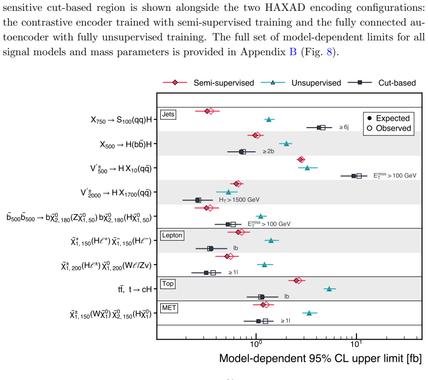
On the paper's own terms, the central discovery is that the HAXAD pipeline—feature embedding, CATHODE sideband-interpolation background estimation, and CWoLa weakly supervised classification—can be extended into a complete search framework competitive with dedicated cut-based analyses. The key empirical result is that with two new encoders, a signal-agnostic variational autoencoder and a semi-supervised contrastive encoder, the method matches or exceeds the best individual cut-based limits for a wide variety of the considered signal models at an integrated luminosity of 470 inverse femtobarns. The paper also establishes that model-dependent cross-section limits must be obtained through a sig
What carries the argument
The load-bearing mechanism is the three-stage HAXAD chain. Stage one embeds event observables into a low-dimensional latent space using either a variational autoencoder (unsupervised) or a contrastive encoder with a transformer-based neural network (semi-supervised). Stage two models the non-resonant background with a normalizing flow—a generative density model—conditioned on the diphoton invariant mass, trained in the Higgs mass sidebands and interpolated into the signal region (CATHODE), while the resonant Standard Model Higgs component is added from simulation. Stage three applies the CWoLa principle: classification without labels, where boosted decision trees trained to separate pseudo-d
Load-bearing premise
The whole background estimate collapses if the non-resonant background's latent-space distribution is not smooth between the Higgs mass sidebands and the signal region, because then the weakly supervised classifier would learn background mismodeling rather than new physics.
What would settle it
Run the full pipeline on a background-only pseudo-dataset in which the continuum background's latent-space density is artificially given a sharp step or a strong slope change across the 120-130 GeV mass window; if the fitted 125 GeV signal yield exceeds the spurious-signal tolerance max|N_sp| <= 0.2*delta_125 + 2*sigma_125 for the chosen background function, the smooth-interpolation assumption is falsified.
If this is right
- A single HAXAD analysis can set a model-independent 95% CL upper limit on any new-physics signal containing a Standard-Model-like H to gamma gamma decay, with no signal-specific optimization.
- For many benchmark models the data-driven pipeline is as strong as or stronger than the best manually designed cut region, suggesting generic searches need not sacrifice sensitivity to remain agnostic.
- The semi-supervised contrastive encoder is the most sensitive configuration and retains most of its performance on signal mass points held out from training, while the unsupervised encoder offers a fully agnostic but weaker alternative.
- Model-dependent limits require the signal-injection calibration procedure, and the paper provides such limits for every benchmark signal and mass point—the ingredient a future search would need to interpret an excess.
- The complete inference framework, including spurious-signal control and expected-limit bands, is worked out for a 470 inverse femtobarn dataset, moving the method from proof-of-principle toward application to recorded collider data.
Where Pith is reading between the lines
- Editorial inference: the smooth sideband-to-signal-region interpolation means HAXAD will be most powerful for anomalies whose associated objects produce slowly varying latent features; a signal that creates a sharp latent-space boundary at the mass-window edge could be missed or mistaken for background mismodeling.
- Editorial inference: because the semi-supervised encoder trains on many labeled processes, its performance on a genuinely new signal likely depends on how close that signal sits to the training mix; a systematic hold-out study across entire theory classes would map this dependence.
- Editorial inference: the same three-stage design could be transplanted to other Higgs decay channels, where the mass resolution and the smoothness of the non-resonant background differ; the optimal choice of decay mode is a testable design question rather than a fixed property.
- Editorial inference: a real-data application will require validating the background estimate against data in an unblinded control region, since the demonstrator uses simulated data for both the observations and the background model; the gap between simulated and real detector response remains the main open question for deployment.
Editorial analysis
A structured set of objections, weighed in public.
Referee Report
Summary. This paper extends the HAXAD anomaly-detection strategy for searches of new physics in events with an SM-like Higgs boson decaying to two photons. The analysis proceeds in three ML stages: an embedding stage (either an unsupervised VAE or a semi-supervised contrastive encoder), a CATHODE-style background-estimation stage in which a normalizing flow is trained on the Higgs mass sidebands and interpolated into the signal region, and a weakly supervised CWoLa classifier that distinguishes pseudo-data from the estimated background. A new statistical framework derives a model-independent 95% CL upper limit on the number of excess Higgs-like events and converts it into model-dependent cross-section limits via a signal-injection efficiency calibration. The method is benchmarked on a wide set of simulated BSM signal processes at 470 fb^-1 and compared with single cut-based regions inspired by the ATLAS Run 2 model-independent H->gamma gamma search. The central claim is that HAXAD matches or exceeds the best individual cut-based limits for a wide variety of considered signal models.
Significance. If the claims hold, this is a valuable step toward deploying ML-based anomaly detection in a Higgs-associated final state at the LHC. The paper is technically rich: it provides detailed descriptions of the encoder architectures, the normalizing flow, the CWoLa classifier, the spurious-signal test, bootstrap averaging over classifier ensembles, and the injection-calibrated limit-setting procedure. The cut-based comparison is conservative in that the most sensitive individual cut-based region is selected for each signal. The authors also include an appendix probing interpolation and extrapolation of the semi-supervised encoder, which is exactly the kind of check needed for a credible anomaly-detection claim. However, the two main load-bearing points -- the unbiasedness of the CATHODE background estimate in the joint latent space, and the generality of the semi-supervised encoder to signals not used in training -- are not yet validated to the level required by the paper's headline claim. Both issues are addressable with additional closure and held-out tests.
major comments (2)
- [3.2, Appendix A, Eq. (3.2)] The load-bearing assumption of the paper is stated in Sec. 3.2: the non-resonant component is 'assumed to vary smoothly between the SB and the SR' and is learned in the SB and interpolated into the SR. This assumption is not validated in the joint latent space that the classifier actually uses. Appendix A (Figs. 5 and 6) shows only one-dimensional marginal projections of the latent features. A normalizing flow can reproduce marginals while mis-modeling the joint conditional density p(z|m_gamma_gamma) in the SR. Since the BDT of Sec. 3.3 uses all latent dimensions jointly, any such mismatch would make the classifier output reflect background mismodeling rather than signal. The spurious-signal test in Sec. 3.4 checks only the selected m_gamma_gamma spectrum, so it cannot detect a latent-space mismatch that shifts the score threshold without creating a mass peak. The model-independent limit
- [3.1.2, 4.1, 4.2, Fig. 4, Appendix C] The central claim that HAXAD 'matches or exceeds the best individual cut-based limits for a wide variety of considered signal models' is made for benchmark models that were used in training the semi-supervised encoder at the same mass points. The paper itself notes in Sec. 4.1 that sensitivity is larger for trained signals, and Appendix C performs held-out tests for only two cases: one interpolation (chi+/- 400) and one extrapolation (V' to X300). The extrapolation test shows a degradation from 1.47 fb^-1 to 3.24 fb^-1, evidence of robustness for one hadronic/MET-like signal but not a broad validation. For the jets, top, and lepton classes in Fig. 4, the benchmark points are not held out. To support the anomaly-detection claim, either restrict the headline claim to the unsupervised encoder or to genuinely unseen signals, or provide a version of Fig. 4 in which every signal category is ex
minor comments (5)
- [Fig. 2, Sec. 3.4] The y-axis label 'Signal yield after cut [a.u.]' in Fig. 2 conflicts with Sec. 3.4, where the yield is determined from generator-level labels and should have physical units. Please make the units consistent.
- [Eq. (3.1), Sec. 3.1.2] The KL notation N(0,0.1) is ambiguous; please specify whether 0.1 is the variance or the standard deviation of the Gaussian prior.
- [Sec. 1, Table 1, Fig. 8] The text says '12 simulated signal models' but Table 1 and Fig. 8 list many mass points per process. Please clarify whether 'signal models' means benchmark process classes or individual mass points.
- [Sec. 3.2] In the demonstrator, the exponential fit to m_gamma_gamma is performed on the full spectrum, while in real data it would be SB-only. This difference can affect the conditional flow through the sampled m_gamma_gamma values; it should be explicitly listed as a caveat in the main text, not only in the methodological description.
- [Appendix C] The sentence about reaching 'the discovery threshold with an initial signal strength of less than 1 sigma' appears to summarize results from Ref. [43] rather than from this paper; please state this explicitly or quantify it in the present context.
Circularity Check
Semi-supervised encoder is benchmarked on the same signal models used to train it; Eq. (3.1) directly optimizes the latent separation that the SIC and limit comparisons then measure.
specific steps
-
fitted input called prediction
[Sec. 3.1.2 (contrastive encoder training), Sec. 4.1-4.2 (Figs. 3, 4), App. C]
"During model training, Monte Carlo (MC) samples from all processes listed in Table 1 are used. ... Nevertheless, its sensitivity remains larger for the signal models which are used in the training."
The contrastive loss in Eq. (3.1) explicitly pulls events of the same process together and pushes events of different processes apart, so for every Table 1 benchmark signal the latent-space separation is itself the training target. Reporting SIC and model-dependent limits on those same benchmarks is therefore an in-sample evaluation: high sensitivity is substantially a consequence of the training objective, not an independent anomaly-detection prediction. The paper confirms this by stating that sensitivity is larger for trained signals, and App. C shows the effect quantitatively (the V' observed limit degrades from 1.47 fb^-1 to 3.24 fb^-1 when the full process is held out). Thus the headline 'matches or exceeds cut-based limits for a wide variety of considered signal models' is partly for
full rationale
The core derivation chain—CATHODE background estimation interpolating the non-resonant component from sidebands to the signal region, CWoLa weakly supervised classification against that background estimate, and the binned-likelihood inference with spurious-signal test and signal-injection calibration—is self-contained and does not reduce by construction to its inputs. The model-independent limit is measured from pseudo-data, and the model-dependent cross-section limit is defined explicitly as the crossing of the injection curve with that limit, so the statistical machinery is not circular. The background smoothness assumption in Sec. 3.2 is a substantive physical ansatz, not a fitted prediction; its closure is tested in App. A, albeit only via one-dimensional projections, which is a validation-depth concern rather than a circularity. The main circular element is the semi-supervised contrastive encoder: it is trained with labels for all benchmark signals in Table 1, and the SIC and limit results in Figs. 3-4 are then reported for those same signals. Because Eq. (3.1) directly optimizes process separation, the measured sensitivity on those signals is in-sample by construction. The paper discloses this and provides an extrapolation test in App. C, and the unsupervised VAE remains fully signal-agnostic, so the central claim retains independent content. No load-bearing self-citation chain or imported uniqueness theorem is present; the method rests on published external methods (CWoLa, CATHODE) plus locally demonstrated extensions. Overall the analysis is largely non-circular, with a partial in-sample evaluation penalty for the semi-supervised variant.
Axiom & Free-Parameter Ledger
free parameters (6)
- VAE KL weight beta =
0.1
- Contrastive loss temperature tau and KL weight lambda =
tau=0.1, lambda=0.1
- Latent dimensionality =
7 (unsupervised), 6 (semi-supervised)
- Classifier selection working point epsilon_B =
0.05% of estimated background retained
- Spurious-signal acceptance criterion =
max|N_sp| <= 0.2*delta_125 + 2*sigma_125 and chi^2/ndf < 3
- Flow and BDT architecture hyperparameters =
six RQS layers, 10 bins; 50 trees, depth 5, learning rate 0.01
axioms (5)
- standard math CWoLa theorem: a classifier trained on mixed data versus estimated background converges to the optimal signal-versus-background classifier given a correct background model and infinite data.
- domain assumption Non-resonant background distribution in latent space is smooth in m_gamma_gamma and interpolable from sidebands into the signal region.
- domain assumption Pseudo-data built by unweighting MC samples at 470 fb^-1 faithfully represents what recorded LHC data would look like.
- domain assumption SM Higgs resonant background can be modeled by MC and its yield N_H fixed in the final fit.
- domain assumption Signal-injection crossing-point calibration yields valid coverage for mild excesses (approximately up to 3 sigma).
read the original abstract
The Higgs boson, with its universal coupling to mass, provides a broadly applicable portal to sectors beyond the Standard Model and is therefore a natural anchor for anomaly detection (AD) at collider experiments. The Higgs And X Anomaly Detection (HAXAD) strategy offers a principled approach to searching for such anomalies occurring in association with a Higgs boson by combining machine-learning-based feature embedding, background estimation, and weakly supervised classification. This work extends the previous HAXAD approach towards the level of maturity required for application to recorded collider data. A major addition is the introduction and comparison of two new embedding strategies, which in turn shape the background estimation and classification. In addition, a new inference framework is developed, yielding signal-agnostic and signal-specific cross section limits and thereby completing the statistical machinery needed for future AD analyses built on HAXAD. The set of investigated signal models is also significantly expanded, allowing for the evaluation of sensitivity on a much broader phase space. Improvements to the method increase signal sensitivity with respect to the original method, and when benchmarked against an example cut-based search on the same final state, HAXAD matches or exceeds the best individual cut-based limits for a wide variety of considered signal models. These developments strengthen the case for HAXAD as a viable and compelling AD-based search strategy with novel discovery potential at colliders.
Figures




Reference graph
Works this paper leans on
-
[1]
Boveia and C
A. Boveia and C. Doglioni,Dark matter searches at colliders,Annual Review of Nuclear and Particle Science68(2018) 429–459
2018
-
[2]
Craig,Naturalness: past, present, and future,Eur
N. Craig,Naturalness: past, present, and future,Eur. Phys. J. C83(2023) 825 [2205.05708]
Pith/arXiv arXiv 2023
-
[3]
Belis, P
V. Belis, P. Odagiu and T.K. Aarrestad,Machine learning for anomaly detection in particle physics,Reviews in Physics12(2024) 100091
2024
-
[4]
Karagiorgi, G
G. Karagiorgi, G. Kasieczka, S. Kravitz, B. Nachman and D. Shih,Machine learning in the search for new fundamental physics,Nature Reviews Physics4(2022) 399
2022
-
[5]
Kasieczka, B
G. Kasieczka, B. Nachman, D. Shih, O. Amram, A. Andreassen, K. Benkendorfer et al.,The LHC Olympics 2020 a community challenge for anomaly detection in high energy physics, Reports on Progress in Physics84(2021) 124201
2020
-
[6]
Aarrestad, M
T. Aarrestad, M. van Beekveld, M. Bona, A. Boveia, S. Caron, J. Davies et al.,The dark machines anomaly score challenge: Benchmark data and model independent event classification for the large hadron collider,SciPost Physics12(2022)
2022
-
[7]
B. Patt and F. Wilczek,Higgs-field portal into hidden sectors,hep-ph/0605188
-
[8]
M. Farina, Y. Nakai and D. Shih,Searching for New Physics with Deep Autoencoders,Phys. Rev. D101(2020) 075021 [1808.08992]
Pith/arXiv arXiv 2020
-
[9]
T. Heimel, G. Kasieczka, T. Plehn and J.M. Thompson,QCD or What?,SciPost Phys.6 (2019) 030 [1808.08979]
Pith/arXiv arXiv 2019
-
[10]
E.M. Metodiev, B. Nachman and J. Thaler,Classification without labels: Learning from mixed samples in high energy physics,JHEP10(2017) 174 [1708.02949]. – 18 –
Pith/arXiv arXiv 2017
-
[11]
Collins, K
J. Collins, K. Howe and B. Nachman,Anomaly detection for resonant new physics with machine learning,Phys. Rev. Lett.121(2018)
2018
-
[12]
Collins, K
J.H. Collins, K. Howe and B. Nachman,Extending the search for new resonances with machine learning,Phys. Rev. D99(2019)
2019
-
[13]
M. Kuusela, T. Vatanen, E. Malmi, T. Raiko, T. Aaltonen and Y. Nagai,Semi-Supervised Anomaly Detection - Towards Model-Independent Searches of New Physics,J. Phys. Conf. Ser.368(2012) 012032 [1112.3329]
Pith/arXiv arXiv 2012
-
[14]
S.E. Park, D. Rankin, S.-M. Udrescu, M. Yunus and P. Harris,Quasi Anomalous Knowledge: Searching for new physics with embedded knowledge,JHEP06(2021) 030 [2011.03550]
Pith/arXiv arXiv 2021
-
[15]
ATLAS Collaboration,Anomaly detection search for new resonances decaying into a higgs boson and a generic new particlexin hadronic final states using √s= 13 TeVppcollisions with the atlas detector,Phys. Rev. D108(2023) 052009
2023
-
[16]
ATLAS Collaboration,Weakly supervised anomaly detection for resonant new physics in the dijet final state using proton-proton collisions at √s= 13 tev with the atlas detector,Phys. Rev. D112(2025) 072009
2025
-
[17]
ATLAS Collaboration,Search for new phenomena in two-body invariant mass distributions using unsupervised machine learning for anomaly detection at √s= 13 TeVwith the atlas detector,Phys. Rev. Lett.132(2024) 081801
2024
-
[18]
CMS Collaboration,Model-agnostic search for dijet resonances with anomalous jet substructure in proton–proton collisions at √s= 13 tev,Reports on Progress in Physics88 (2025) 067802
2025
-
[19]
C.L. Cheng, S. Demers, S. Diefenbacher, R. Li, B. Nachman and D. Noll,Weakly supervised anomaly detection in events with a higgs boson and exotic physics,Phys. Rev. D114(2026) 012003. [20]ATLAScollaboration,Model-independent search for the presence of new physics in events includingH→γγwith √s= 13 TeV pp data recorded by the ATLAS detector at the LHC, JHE...
Pith/arXiv arXiv 2026
-
[21]
A. Hallin, J. Isaacson, G. Kasieczka, C. Krause, B. Nachman, T. Quadfasel et al.,Classifying anomalies through outer density estimation,Phys. Rev. D106(2022) 055006 [2109.00546]
Pith/arXiv arXiv 2022
-
[22]
J. Alwall, R. Frederix, S. Frixione, V. Hirschi, F. Maltoni, O. Mattelaer et al.,The automated computation of tree-level and next-to-leading order differential cross sections, and their matching to parton shower simulations,JHEP07(2014) 079 [1405.0301]
Pith/arXiv arXiv 2014
-
[23]
Bierlich, S
C. Bierlich, S. Chakraborty, N. Desai, L. Gellersen, I. Helenius, P. Ilten et al.,A comprehensive guide to the physics and usage of pythia 8.3,SciPost Phys. Codebases(2022) 8
2022
-
[24]
Bierlich, S
C. Bierlich, S. Chakraborty, N. Desai, L. Gellersen, I. Helenius, P. Ilten et al.,Codebase release 8.3 for pythia,SciPost Phys. Codebases(2022) 8
2022
-
[25]
M.L. Mangano, M. Moretti, F. Piccinini and M. Treccani,Matching matrix elements and shower evolution for top-quark production in hadronic collisions,JHEP01(2007) 013 [hep-ph/0611129]
Pith/arXiv arXiv 2007
-
[26]
J. Alwall et al.,Comparative study of various algorithms for the merging of parton showers and matrix elements in hadronic collisions,Eur. Phys. J. C53(2008) 473 [0706.2569]. – 19 – [27]DELPHES 3collaboration,DELPHES 3, A modular framework for fast simulation of a generic collider experiment,JHEP02(2014) 057 [1307.6346]
Pith/arXiv arXiv 2008
-
[28]
M. Cacciari, G.P. Salam and G. Soyez,The anti-k t jet clustering algorithm,JHEP04(2008) 063 [0802.1189]
Pith/arXiv arXiv 2008
-
[29]
M. Cacciari, G.P. Salam and G. Soyez,FastJet User Manual,Eur. Phys. J. C72(2012) 1896 [1111.6097]
Pith/arXiv arXiv 2012
-
[30]
T. Robens, T. Stefaniak and J. Wittbrodt,Two-real-scalar-singlet extension of the SM: LHC phenomenology and benchmark scenarios,Eur. Phys. J. C80(2020) 151 [1908.08554]
Pith/arXiv arXiv 2020
-
[31]
P. Basler, S. Dawson, C. Englert and M. M¨ uhlleitner,Showcasing HH production: Benchmarks for the LHC and HL-LHC,Phys. Rev. D99(2019) 055048 [1812.03542]
Pith/arXiv arXiv 2019
-
[32]
S. Baum and N.R. Shah,Benchmark Suggestions for Resonant Double Higgs Production at the LHC for Extended Higgs Sectors,1904.10810
Pith/arXiv arXiv 1904
-
[33]
Z. Chacko, Y. Nomura, M. Papucci and G. Perez,Natural little hierarchy from a partially goldstone twin Higgs,JHEP01(2006) 126 [hep-ph/0510273]
Pith/arXiv arXiv 2006
-
[34]
G.C. Branco, P.M. Ferreira, L. Lavoura, M.N. Rebelo, M. Sher and J.P. Silva,Theory and phenomenology of two-Higgs-doublet models,Phys. Rept.516(2012) 1 [1106.0034]
Pith/arXiv arXiv 2012
-
[35]
D. Pappadopulo, A. Thamm, R. Torre and A. Wulzer,Heavy Vector Triplets: Bridging Theory and Data,JHEP09(2014) 060 [1402.4431]
Pith/arXiv arXiv 2014
-
[36]
Martin,A Supersymmetry primer,Adv
S.P. Martin,A Supersymmetry primer,Adv. Ser. Direct. High Energy Phys.18(1998) 1 [hep-ph/9709356]
Pith/arXiv arXiv 1998
-
[37]
Barbier et al.,R-parity violating supersymmetry,Phys
R. Barbier et al.,R-parity violating supersymmetry,Phys. Rept.420(2005) 1 [hep-ph/0406039]
Pith/arXiv arXiv 2005
-
[38]
Alves et al.,Simplified Models for LHC New Physics Searches,J
D. Alves et al.,Simplified Models for LHC New Physics Searches,J. Phys. G39(2012) 105005 [1105.2838]
Pith/arXiv arXiv 2012
-
[39]
J.A. Aguilar-Saavedra,Top flavor-changing neutral interactions: Theoretical expectations and experimental detection,Acta Phys. Polon. B35(2004) 2695 [hep-ph/0409342]. [40]ATLAScollaboration,Measurement of the properties of Higgs boson production at √s= 13 TeV in theH→γγchannel using139fb −1 ofppcollision data with the ATLAS experiment, JHEP07(2023) 088 [2...
Pith/arXiv arXiv 2004
- [41]
-
[42]
D.P. Kingma and J. Ba,Adam: A method for stochastic optimization,1412.6980
-
[43]
R. Li, B. Nachman and D. Noll,Signal-aware contrastive latent spaces for anomaly detection, 2603.25794
-
[44]
A. Vaswani, N. Shazeer, N. Parmar, J. Uszkoreit, L. Jones, A.N. Gomez et al.,Attention Is All You Need, inAdvances in Neural Information Processing Systems 30, 2017 [1706.03762]
Pith/arXiv arXiv 2017
-
[45]
H. Qu, C. Li and S. Qian,Particle Transformer for Jet Tagging,2202.03772
-
[46]
J. Thaler and K. Van Tilburg,Identifying Boosted Objects with N-subjettiness,JHEP03 (2011) 015 [1011.2268]
Pith/arXiv arXiv 2011
-
[47]
T. Chen, S. Kornblith, M. Norouzi and G. Hinton,A simple framework for contrastive learning of visual representations,2002.05709. – 20 –
Pith/arXiv arXiv 2002
-
[48]
P. Khosla, P. Teterwak, C. Wang, A. Sarna, Y. Tian, P. Isola et al.,Supervised contrastive learning,2004.11362
Pith/arXiv arXiv 2004
-
[49]
I. Loshchilov and F. Hutter,Decoupled weight decay regularization,1711.05101
-
[50]
I. Loshchilov and F. Hutter,SGDR: Stochastic Gradient Descent with Warm Restarts, in International Conference on Learning Representations, 2017 [1608.03983]
Pith/arXiv arXiv 2017
-
[51]
G. Papamakarios, E. Nalisnick, D.J. Rezende, S. Mohamed and B. Lakshminarayanan, Normalizing Flows for Probabilistic Modeling and Inference,J. Machine Learning Res.22 (2021) 2617 [1912.02762]
Pith/arXiv arXiv 2021
-
[52]
C. Durkan, A. Bekasov, I. Murray and G. Papamakarios,Neural spline flows,1906.04032
Pith/arXiv arXiv 1906
-
[53]
M. Germain, K. Gregor, I. Murray and H. Larochelle,MADE: Masked Autoencoder for Distribution Estimation, inProceedings of the 32nd International Conference on Machine Learning, vol. 37 ofProceedings of Machine Learning Research, pp. 881–889, 2015 [1502.03509]
Pith/arXiv arXiv 2015
-
[54]
A. Paszke, S. Gross, F. Massa, A. Lerer, J. Bradbury, G. Chanan et al.,PyTorch: An Imperative Style, High-Performance Deep Learning Library, inAdvances in Neural Information Processing Systems 32, pp. 8024–8035, 2019 [1912.01703]
Pith/arXiv arXiv 2019
-
[55]
nflows: normalizing flows in pytorch
C. Durkan, A. Bekasov, I. Murray and G. Papamakarios, “nflows: normalizing flows in pytorch.” 10.5281/zenodo.4296287, Nov., 2020
-
[56]
T. Finke, M. Hein, G. Kasieczka, M. Kr¨ amer, A. M¨ uck, P. Prangchaikul et al.,Tree-based algorithms for weakly supervised anomaly detection,Phys. Rev. D109(2024) 034033 [2309.13111]
Pith/arXiv arXiv 2024
-
[57]
M. Freytsis, M. Perelstein and Y.C. San,Anomaly detection in the presence of irrelevant features,JHEP02(2024) 220 [2310.13057]
Pith/arXiv arXiv 2024
-
[58]
Friedman,Greedy function approximation: A gradient boosting machine.,Annals Statist
J.H. Friedman,Greedy function approximation: A gradient boosting machine.,Annals Statist. 29(2001) 1189
2001
-
[59]
Chen and C
T. Chen and C. Guestrin,Xgboost: A scalable tree boosting system, inProceedings of the 22nd ACM SIGKDD International Conference on Knowledge Discovery and Data Mining, KDD ’16, pp. 785–794, Association for Computing Machinery, 2016, DOI
2016
-
[60]
E. Gross and O. Vitells,Trial factors for the look elsewhere effect in high energy physics, Eur. Phys. J. C70(2010) 525 [1005.1891]
Pith/arXiv arXiv 2010
-
[61]
ATLAS Collaboration,Recommendations for the Modeling of Smooth Backgrounds, Tech. Rep. ATL-PHYS-PUB-2020-028, CERN, Geneva (2020)
2020
-
[62]
Read,Presentation of search results: TheCL s technique,J
A.L. Read,Presentation of search results: TheCL s technique,J. Phys. G28(2002) 2693
2002
-
[63]
G. Cowan, K. Cranmer, E. Gross and O. Vitells,Asymptotic formulae for likelihood-based tests of new physics,Eur. Phys. J. C71(2011) 1554 [1007.1727]
Pith/arXiv arXiv 2011
-
[64]
T. Finke, M. Kr¨ amer, A. Morandini, A. M¨ uck and I. Oleksiyuk,Autoencoders for unsupervised anomaly detection in high energy physics,2104.09051
-
[65]
K. Fraser, S. Homiller, R.K. Mishra, B. Ostdiek and M.D. Schwartz,Challenges for unsupervised anomaly detection in particle physics,JHEP03(2022) 066 [2110.06948]. – 21 – A Input and Embedded Features The feature distributions in the latent space constructed by the unsupervised (semi-supervised) encoder are shown in fig. 5 (fig. 6). Since reparameterizatio...
Pith/arXiv arXiv 2022
-
[66]
˜χ0 2,150(H˜χ0 1) is included in both figures to illustrate the separation between signal and background in the latent space. In figs. 5c, 5e, 6c and 6e, the signal distribution deviates strongly from the background distribution, creating the overdensity that the weakly supervised classifiers can exploit if such signal events are present in the data. 3 2 ...
-
[67]
The back- ground includes both the non-resonant and the resonant SM Higgs boson components
signal (red) are compared. The back- ground includes both the non-resonant and the resonant SM Higgs boson components. – 22 – 0.3 0.2 0.1 0.0 0.1 0.2 0.3 Latent Dimension 0 10 4 10 3 10 2 10 1 100 101 Fraction of Events / 0.028 Generated Background Signal (a) 0.3 0.2 0.1 0.0 0.1 0.2 0.3 Latent Dimension 1 10 4 10 3 10 2 10 1 100 101 Fraction of Events / 0...
-
[68]
The back- ground includes both the non-resonant and the resonant SM Higgs boson components
signal (red) are compared. The back- ground includes both the non-resonant and the resonant SM Higgs boson components. B Additional Cross Section Limits Figure 7 shows the model-independent cross section limits for the unsupervised and semi- supervised-based HAXAD analyses, compared to several cut-based regions. Figure 8 extends the summary in section 4.2...
2000
-
[69]
0 2, 150(H 0 1) ± 1, 200(W 0
-
[70]
0 2, 200(H 0 1) ± 1, 300(W 0
-
[71]
0 2, 300(H 0 1) ± 1, 600(W 0
-
[72]
Filled markers with their±1σ bands show the expected limits and open markers the observed limits
0 2, 600(H 0 1) 2b 6j 2b 2b 2b Emiss T > 100 GeV tophad Emiss T > 100 GeV HT > 1000 GeV HT > 1500 GeV Emiss T > 100 GeV Emiss T > 200 GeV Emiss T > 200 GeV Emiss T > 300 GeV Emiss T > 300 GeV Emiss T > 300 GeV lb lb lb 1l 1l Emiss T > 200 GeV lb lb lb lb lb Emiss T > 200 GeV Emiss T > 200 GeV 1l Emiss T > 100 GeV Emiss T > 200 GeV Emiss T > 300 GeV Jets L...
2000
discussion (0)
Sign in with ORCID, Apple, or X to comment. Anyone can read and Pith papers without signing in.