REVIEW 4 minor 35 references
Is Memorization Helpful or Harmful? Prior Information Sets the Threshold
T0 review · 0 major / 4 minor · reviewed 2026-08-03 · deepseek-v4-flash
Pith's one-line read In an overparameterized Bayesian linear model, the prior's Fisher information and variance set exact thresholds: below 1/J_pi optimal estimators must memorize, above V_pi they must avoid overfitting.
desk verdict A genuinely clarifying threshold result for Bayesian linear regression that reconciles the memorization-necessary and overfitting-harmful camps; the proof core holds up on inspection, with one minor gap in a side asymptotic. read the letter →
The pith
A machine-rendered reading of the paper's core claim, the machinery that carries it, and where it could break.
The reading
What carries the argument
The load-bearing object is the Fisher information of the noised pushed-forward distribution, J(sigma^2) = (1/n) E_{y ~ pi' * N(0, sigma^2 I)}[||nabla log p_sigma^2(y)||^2], related to the Bayes training error exactly by Train(theta_hat_B) = sigma^4 * J(sigma^2) through Tweedie's formula. The proof combines Stam's Fisher information inequality, which yields J(sigma^2) <= (J_pi^{-1} + sigma^2)^{-1}, and a Cramer-Rao/variance bound, which yields J(sigma^2) >= (V_pi + sigma^2)^{-1} after a Cauchy-Schwarz integration-by-parts identity, plus lower-semicontinuity of Fisher information to control the sigma^2 -> 0 limit. This identity converts training error into a purely information-theoretic quanti
What would settle it
Fix any prior with positive differentiable density and any full-row-rank design X; compute Train(theta_hat_B) for many noise levels and check whether sigma^4/(V_pi + sigma^2) <= Train(theta_hat_B) <= sigma^4/(J_pi^{-1} + sigma^2) for all sigma^2. A single violation, or a failure of Train(theta_hat_B)/sigma^4 to tend to J_pi as sigma^2 goes to 0, would refute Theorem 1. Alternatively, in the regime sigma^2 <= J_pi^{-1}, find a near-optimal estimator whose excess risk is small but whose training error is not o(sigma^2).
Extended reading notes
Core claim
Treating y = X*theta + sigma*tau with theta drawn from a prior pi that has a positive differentiable density, the discovery is that optimal generalization is tied to training error through the two prior parameters J_pi = E[||nabla log p(X*theta)||^2/n | X] and V_pi = E[||X*theta||^2/n | X]. Theorem 1 sandwiches the Bayes estimator's mean squared training error between sigma^4/(V_pi + sigma^2) and sigma^4/(J_pi^{-1} + sigma^2). The asymptotic directions show Train(theta_hat_B) = J_pi*sigma^4 + o(sigma^4) as sigma^2 -> 0, and Train(theta_hat_B) = sigma^2 - V_pi + o(1) as sigma^2 -> infinity. Since the posterior mean is the unique prediction-optimal estimator (Proposition 1), any near-optimal e
Load-bearing premise
Everything is measured against the Bayes estimator under the true prior pi, and pi is required to have a positive, differentiable density; if the practitioner's prior is misspecified or the prior puts mass on a lower-dimensional set, the two thresholds describe the wrong benchmark and the memorization/overfitting verdicts need not hold.
Editorial extensions
If this is right
- If the sandwich holds, an uninformative prior with J_pi and V_pi of order 1 puts any positive-but-small noise in the memorization regime: near-optimal estimators must have training error o(sigma^2).
- If the prior is concentrated near a low-dimensional manifold, J_pi^{-1} is tiny, so for fixed noise memorization is not forced; overfitting becomes harmful once sigma^2 >= V_pi.
- For any C > 1, an estimator with Train >= C*J_pi*sigma^4 in the low-noise regime suffers excess prediction risk linear in its training error; an estimator with Train <= sigma^2 - C*V_pi in the high-noise regime suffers excess risk quadratic in the overfit amount divided by sigma^2.
- The Bayes-optimal training error increases monotonically with noise, while Train/sigma^4 decreases, so the transition from memorization-necessary to overfitting-harmful is a continuous shift rather than a sharp phase flip.
- Exact low-rank priors without a density sit outside the main theorem; direct computation gives Train(theta_hat_B) -> sigma^2*(1-rho) + O(sigma^4), so bounded overfitting is harmless there.
Reading between the lines
- If these thresholds are robust, a practitioner could estimate J_pi and V_pi from the prior or from score statistics of the posterior and decide whether to regularize or interpolate before seeing data; the paper does not develop this diagnostic.
- The Bayesian benchmark assumes the true prior is known. For a misspecified prior, the same sandwich may bound the training error of the misspecified-Bayes estimator against the wrong optimum, so the necessity and harm statements would not transfer unchanged; this is an extension question the paper leaves open.
- Because a positive density is required, the memorization regime at extremely small noise can be an artifact of local flatness even under strongly structured priors; replacing the density condition with atom-containing or exactly low-rank priors may remove that regime and change the practical advice.
- The same Fisher-information identity suggests a finite-sample check: for a fixed design and prior, compute Train(theta_hat_B) = sigma^4 * J(sigma^2) numerically for several noise levels and compare against the sandwich; a sizable violation would indicate the core theorem is not capturing the true training error.
Signed reviews
Editorial analysis
A structured set of objections, weighed in public.
Referee Report
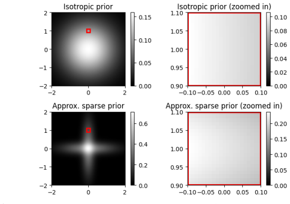
Summary. The paper studies the Bayesian linear model y = Xθ + στ with d ≥ n and a fixed, known prior π on θ. It introduces two prior-dependent quantities, the Fisher information Jπ and the variance Vπ of the push-forward distribution of Xθ, and proves a non-asymptotic sandwich for the training error of the Bayes estimator: σ⁴/(Vπ+σ²) ≤ Train(θ̂_B) ≤ σ⁴/(Jπ^{-1}+σ²) (Theorem 1). Combining this with a Pythagorean decomposition for arbitrary estimators (Proposition 1), it derives two threshold laws: when σ² ≤ Jπ^{-1}, any near-optimal estimator must have training error at most O(Jπσ⁴) = o(σ²), so memorization is necessary (Corollary 2.1); when σ² ≥ Vπ, any near-optimal estimator must have training error at least σ² − Vπ, so overfitting is harmful (Corollary 2.2). The main theorem is non-asymptotic; Section 3 illustrates the thresholds in isotropic Gaussian, approximately low-rank Gaussian, and approximately sparse mixture priors using random matrix asymptotics. Appendices supply proofs and supporting lemmas.
Significance. If correct, the paper gives a clean conceptual unification: memorization and harmful overfitting are not contradictory phenomena but two regimes of a single threshold law set by the prior. The thresholds Jπ^{-1} and Vπ are derived, not fitted; the proof uses classical tools (Cramér–Rao, Stam's Fisher information inequality, lower semicontinuity of Fisher information) and the core bound holds for fixed d and n without asymptotic assumptions. The paper is explicit about its scope (known prior, positive differentiable density) and honestly flags the artifact that exact low-rank/sparse priors are excluded from the main theorem. Strengths include the non-asymptotic nature of Theorem 1, the concrete random-matrix examples, and the availability of reproducible simulation code. The contribution is likely to be of broad interest to the high-dimensional statistics and learning theory communities.
minor comments (4)
- [Appendix B.2, Part III (high-noise asymptotic)] The dominated-convergence step for E[θ̂_B θ̂_B^T] is asserted too quickly. The assertion that ∫∥θ∥²π(dθ)<∞ suffices is not by itself enough: the integrand is a ratio whose denominator can be small. A uniform lower bound on the denominator (e.g., using positivity of the density p and the pointwise limit e^{−∥τ∥²/2}) is needed to justify the interchange. This does not affect Corollaries 2.1–2.2, which rely only on the non-asymptotic bounds in Eq. (2), but the proof of Eq. (4) should be completed.
- [§4.2, proof of Proposition 6] The claim that J(σ²)=Train(σ²)/σ⁴ is non-increasing is said to follow from Stam's inequality J(t)^{-1} ≥ J(0)^{-1}+t. That inequality gives a decreasing upper bound on J(t), not monotonicity of J itself. The statement is true, but the correct justification is the derivative formula J'(t)=−E∥∇² log p_t∥²_F/n (Appendix E.2); the proof should be corrected.
- [Appendix B.2, Lemma B.1] The variational characterization of Fisher information is abbreviated. The equality J(t)=sup_b{−2/n∫p_t∇·b − 1/n∫p_t∥b∥²} requires an approximation argument for the choice b=∇log p_t by compactly supported smooth vector fields. The sentence 'ϵ_b can be arbitrarily small' is not a full justification. This affects only the proof of the low-noise l.s.c. step, not the non-asymptotic sandwich.
- [Throughout] Several inline logical symbols and square-root spans are garbled in the submitted PDF (e.g., 'Leftr⫯g⊸tl⫯ne⇒' in Section 2.1 and broken radicals in Theorem 2 and Appendix B.3). Please ensure the final typesetting is clean; this appears to be a rendering artifact rather than a mathematical issue.
Circularity Check
No significant circularity; the threshold bounds are derived, not fitted, and self-citations are not load-bearing.
full rationale
The paper's central derivation is self-contained. Theorem 1's sandwich bound (Eq. 2) is proved in Appendix B.2 from external information-theoretic inequalities: 'The Fisher information upper bound is a direct corollary of Stam's Fisher information inequality in Lemma A.2... The lower bound follows from the classical scalar version of Cramer-Rao bound'. The thresholds J_pi^{-1} and V_pi are prior-defined parameters in Eq. (1), not calibrated to the training errors they predict. The memorization/harm corollaries follow by substituting the Theorem 1 bounds into Proposition 1's Pythagorean cost identity, which is standard Bayes optimality plus Minkowski; this is a deduction, not a renaming. Example limits (Propositions 2-5) are computed from random matrix theory, and the approximately-sparse example is checked against external bounds. Citations to the authors' prior work [12,13,28] are contextual or comparative (e.g., footnote 5 notes the isotropic example is 'the same setup considered in [13]'), but the main theorem does not rest on those papers; the proof cites external results (Stam [34], Dembo-Cover-Thomas [14], Guo et al. [19,20], Ledoux [24]). The only caveat I see is a technical one in the high-noise proof (Appendix B.2, Part III), where dominated convergence for E[theta_hat_B theta_hat_B^T] is asserted too quickly from integral ||theta||^2 pi(dtheta) < infinity; this is a rigor gap, not a circularity, and Eq. (4) is not needed for Corollaries 2.1-2.2. The explicit scope condition (positive differentiable density, known prior pi) is stated, not hidden, and the paper itself flags the small-noise artifact for structured priors in Section 2.4.1. No fitted input is renamed as a prediction, and no uniqueness theorem is imported from the authors' prior work.
Assumptions & free parameters
assumptions (8)
- standard math Tweedie's formula: E[Xθ|y] = y + σ²∇log p_{σ²}(y)
- standard math Stam's Fisher information inequality and the entropic isoperimetric inequality (Lemmas A.2, A.3 from [14,34])
- standard math Cramér-Rao lower bound via Cauchy-Schwarz
- standard math Lower semi-continuity of Fisher information under weak convergence (Lemma B.1)
- standard math Bai-Yin and generalized Marchenko-Pastur laws (Lemmas A.4-A.6)
- domain assumption Prior π has positive, differentiable density on R^d; X full row rank with d ≥ n
- domain assumption The Bayesian model M_X(π,σ²) is the true data-generating mechanism and the prior is known to the statistician
- domain assumption Assumption 1: d/n → γ, i.i.d. standardized design entries with bounded fourth moment
Cite this review
Pith. "Pith review of Is Memorization Helpful or Harmful? Prior Information Sets the Threshold." pith.science (2026). https://pith.science/paper/YLTVMTQR
@misc{pith2026260209405,
  author       = {Pith},
  title        = {Pith review of: Is Memorization Helpful or Harmful? Prior Information Sets the Threshold},
  year         = {2026},
  howpublished = {\url{https://pith.science/paper/YLTVMTQR}},
  note         = {Machine review of arXiv:2602.09405}
}
abstract
We examine the connection between training error and generalization error for arbitrary estimating procedures, working in an overparameterized linear model under general priors in a Bayesian setup. We find determining factors inherent to the prior distribution $\pi$, giving explicit conditions under which optimal generalization necessitates that the training error be (i) near interpolating relative to the noise size (i.e., memorization is necessary), or (ii) close to the noise level (i.e., overfitting is harmful). Remarkably, these phenomena occur when the noise reaches thresholds determined by the Fisher information and the variance parameters of the prior $\pi$.
Figures


Reference graph
Works this paper leans on
-
[1]
Artstein, K
S. Artstein, K. Ball, F. Barthe, and A. Naor. Solution of shannon’s problem on the monotonicity of entropy.Journal of the American Mathematical Society, 17(4):975–982, 2004
2004
-
[2]
Bai and J
Z. Bai and J. W. Silverstein.Spectral analysis of large dimensional random matrices, volume 20. Springer, 2010
2010
-
[3]
Bakry and M
D. Bakry and M. Émery. Diffusions hypercontractives. InSéminaire de Probabilités XIX 1983/84: Proceedings, pages 177–206. Springer, 2006
1983
-
[4]
Bakry, I
D. Bakry, I. Gentil, and M. Ledoux.Analysis and geometry of Markov diffusion operators, volume 348. Springer Science & Business Media, 2013. 12
2013
-
[5]
P. L. Bartlett, P. M. Long, G. Lugosi, and A. Tsigler. Benign overfitting in linear regression. Proceedings of the National Academy of Sciences, 117(48):30063–30070, 2020
2020
-
[6]
Belkin, D
M. Belkin, D. J. Hsu, and P. Mitra. Overfitting or perfect fitting? risk bounds for classification and regression rules that interpolate.Advances in neural information processing systems, 31, 2018
2018
-
[7]
Belkin, A
M. Belkin, A. Rakhlin, and A. B. Tsybakov. Does data interpolation contradict statistical optimality? InThe 22nd international conference on artificial intelligence and statistics, pages 1611–1619. PMLR, 2019
2019
-
[8]
Billingsley.Probability and Measure
P. Billingsley.Probability and Measure. Wiley, 3 edition, 1995
1995
Show all 35 references
-
[9]
S. G. Bobkov, G. P. Chistyakov, and F. Götze. Fisher information and the central limit theorem. Probability theory and related fields, 159(1):1–59, 2014
2014
-
[10]
Candes and B
E. Candes and B. Recht. Exact matrix completion via convex optimization.Communications of the ACM, 55(6):111–119, 2012
2012
-
[11]
E. J. Candes, M. B. Wakin, and S. P. Boyd. Enhancing sparsity by reweightedℓ1 minimization. Journal of Fourier analysis and applications, 14(5):877–905, 2008
2008
-
[12]
Cheng and A
C. Cheng and A. Montanari. Dimension free ridge regression.The Annals of Statistics, 52(6): 2879–2912, 2024
2024
-
[13]
Cheng, J
C. Cheng, J. Duchi, and R. Kuditipudi. Memorize to generalize: on the necessity of interpolation in high dimensional linear regression. InConference on Learning Theory, pages 5528–5560. PMLR, 2022
2022
-
[14]
Dembo, T
A. Dembo, T. M. Cover, and J. A. Thomas. Information theoretic inequalities.IEEE Transactions on Information theory, 37(6):1501–1518, 2002
2002
-
[15]
Dytso, H
A. Dytso, H. V. Poor, and S. S. Shitz. A general derivative identity for the conditional mean estimator in gaussian noise and some applications. In2020 IEEE International Symposium on Information Theory (ISIT), pages 1183–1188. IEEE, 2020
2020
-
[16]
B. Efron. Tweedie’s formula and selection bias.Journal of the American Statistical Association, 106(496):1602–1614, 2011
2011
-
[17]
V. Feldman. Does learning require memorization? a short tale about a long tail. InProceedings of the 52nd annual ACM SIGACT symposium on theory of computing, pages 954–959, 2020
2020
-
[18]
Gunasekar, B
S. Gunasekar, B. E. Woodworth, S. Bhojanapalli, B. Neyshabur, and N. Srebro. Implicit regularization in matrix factorization.Advances in neural information processing systems, 30, 2017
2017
-
[19]
D. Guo, S. Shamai, and S. Verdú. Mutual information and mmse in gaussian channels. In International Symposium onInformation Theory, 2004. ISIT 2004. Proceedings., pages 349–349. IEEE, 2004
2004
-
[20]
D. Guo, Y. Wu, S. S. Shitz, and S. Verdú. Estimation in gaussian noise: Properties of the minimum mean-square error.IEEE Transactions on Information Theory, 57(4):2371–2385, 2011. 13
2011
-
[21]
Hastie, A
T. Hastie, A. Montanari, S. Rosset, and R. J. Tibshirani. Surprises in high-dimensional ridgeless least squares interpolation.Annals of statistics, 50(2):949, 2022
2022
-
[22]
P. J. Huber and E. M. Ronchetti.Asymptotic Minimax Theory for Estimating Location, chapter 4, pages 71–103. John Wiley & Sons, Ltd, 2009. ISBN 9780470434697. doi: https: //doi.org/10.1002/9780470434697.ch4. URL https://onlinelibrary.wiley.com/doi/abs/ 10.1002/9780470434697.ch4
2009 doi
-
[23]
Isserlis
L. Isserlis. On a formula for the product-moment coefficient of any order of a normal frequency distribution in any number of variables.Biometrika, 12(1/2):134–139, 1918
1918
-
[24]
M. Ledoux. Heat flow derivatives and minimum mean-square error in gaussian noise.IEEE Transactions on Information Theory, 62(6):3401–3409, 2016
2016
-
[25]
E. L. Lehmann and G. Casella.Theory of point estimation. Springer, 1998
1998
-
[26]
ridgeless
T. Liang and A. Rakhlin. Just interpolate: Kernel “ridgeless” regression can generalize.The Annals of Statistics, 48(3):1329–1347, 2020
2020
-
[27]
S. Mei, T. Misiakiewicz, and A. Montanari. Generalization error of random feature and kernel methods: Hypercontractivity and kernel matrix concentration.Applied and Computational Harmonic Analysis, 59:3–84, 2022
2022
-
[28]
M. M. Müller, Y. Luo, and R. F. Barber. Are all models wrong? fundamental limits in distribution-free empirical model falsification.arXiv preprint arXiv:2502.06765, 2025
2025 arXiv
-
[29]
Neyshabur
B. Neyshabur. Implicit regularization in deep learning.arXiv preprint arXiv:1709.01953, 2017
2017 arXiv
-
[30]
Petersen.Riemannian geometry
P. Petersen.Riemannian geometry. Springer, 2006
2006
-
[31]
K. Shah, A. Kalavasis, A. R. Klivans, and G. Daras. Does generation require memorization? creative diffusion models using ambient diffusion.arXiv preprint arXiv:2502.21278, 2025
2025
-
[32]
C. E. Shannon. A mathematical theory of communication.The Bell system technical journal, 27(3):379–423, 1948
1948
-
[33]
J. W. Silverstein and S.-I. Choi. Analysis of the limiting spectral distribution of large dimensional random matrices.Journal of Multivariate Analysis, 54(2):295–309, 1995
1995
-
[34]
A. J. Stam. Some inequalities satisfied by the quantities of information of Fisher and Shannon. Information and Control, 2(2):101–112, 1959
1959
-
[35]
Tibshirani
R. Tibshirani. Regression shrinkage and selection via the lasso.Journal of the Royal Statistical Society Series B: Statistical Methodology, 58(1):267–288, 1996. 14 A Technical lemmas In this section, we gather some technical lemmas from existing work, that will be helpful in t...
1996
Reviewed August 3, 2026 · model on record in the stance chip above.
Discussion (0). Continue with ORCID to comment.