REVIEW 3 major objections 5 minor 53 references
Continuum Fractons: Quantization and the Few Body Problem
T0 review · 3 major / 5 minor · reviewed 2026-08-04 · deepseek-v4-flash
Pith's one-line read Quantized two-fracton motion is governed by a Sturm–Liouville operator with a sharp spectral transition at θ=2.
desk verdict Solid two-body quantization of continuum fractons with a sharp θ=2 spectral transition, conditional on an unexamined operator-ordering choice; three-body part is exploratory. read the letter →
The pith
A machine-rendered reading of the paper's core claim, the machinery that carries it, and where it could break.
The reading
What carries the argument
The pair-inertia function K(x) (vanishing as (1−|x|)^θ at boundaries), the Sturm–Liouville operator −d/dx K(x) d/dx, and the unitary Liouville map ξ(x)=∫_0^x ds/√K(s), ψ→(K)^{1/4}ψ, which converts the operator into a standard Schrödinger Hamiltonian with effective potential V(ξ). Because the domain length in ξ equals the classical freezing time, the finite-versus-infinite domain dichotomy produces the θ=2 spectral transition. For the three-body problem the key machinery is the block-diagonal decomposition of the Hamiltonian on the hexagon of reduced coordinates, with matching conditions on internal K=0 lines handled via a dipole-conserving lattice regularization.
What would settle it
For the alternative operator ordering in Eq. (6), compute the two-body spectrum on (−1,1) with K=(1−x²)^θ; if the discrete-to-continuous transition does not occur at θ=2, the central claim fails. Also, a lattice simulation of θ>2 should show the wavepacket reflection time diverging as the lattice spacing goes to zero; a finite extrapolated limit would rule out the edge pile-up.
Extended reading notes
Core claim
The paper's core claim is that quantized, dipole-conserving continuum fractons are governed, at the two-body level, by the Sturm–Liouville operator −d/dx K(x) d/dx on (−1,1), and that the edge behavior K(x)∼(1−|x|)^θ of the pair inertia function K determines the spectral type: for θ<2 the spectrum is discrete (limit-circle case, with a chosen self-adjoint extension), while for θ>2 it is continuous (limit-point case, essentially self-adjoint). This is established with the help of a unitary Liouville transformation to an ordinary Schrödinger problem, which also explains the dynamics: for θ>2 the effective potential vanishes at infinity, incoming waves suffer exponentially suppressed reflection
Load-bearing premise
The entire spectral classification assumes the operator ordering −d/dx K(x) d/dx chosen in Section II.A; the equally natural symmetrized ordering (p̂ᵢ−p̂ⱼ)²K + h.c. adds K-derivative terms and could shift or wash out the θ=2 transition. For θ<2, the discrete spectrum also assumes the specific Kψ'=0 self-adjoint extension.
Editorial extensions
If this is right
- The two-fracton problem is exactly solvable at θ=1 (Legendre) and completely classified by Sturm–Liouville theory for all θ.
- For θ>2, wavepackets incident on a K→0 edge do not reflect; the reflection time diverges in the continuum limit, so the quantum system reproduces the classical freezing/attractor behavior.
- For θ<2, quantum and classical behavior diverge: the discrete spectrum forbids complete separation to the edges, and wavepackets reflect instead of piling up.
- The finite-energy three-body spectrum is dominated by effective two-body strip sectors, each inheriting the θ=2 transition, while the central hexagonal block shows a numerically drifting threshold conjectured to flow to 2.
- Low-energy three-body eigenstates localize on the six classical attractor regions and tunnel between permutations, giving D_6 symmetry multiplets—a quantum signature of classical order-by-disorder.
Reading between the lines
- Inference: If the θ=2 transition is robust to the operator-ordering ambiguity, the edge exponent θ becomes a tunable control parameter for switching a quantum system between localized (discrete) and delocalized (continuous) behavior without disorder—a possible design principle for fractonic quantum simulators.
- Inference: The block-diagonal Krylov-sector structure seen here in the continuum suggests that Hilbert-space fragmentation is not an artifact of lattice discreteness; increasing particle number at finite density may produce a hierarchy of fragmented sectors, possibly suppressing thermalization even at large N in line with the classical result.
- Inference: The wavepacket pile-up at edges for θ>2 is distinct from ordinary quantum reflection; a testable extension is to probe it in cold-atom or trapped-ion emulations of dipole-conserving dynamics by measuring edge density accumulation as a function of θ.
- Inference: The ultralocal field-theory limit (K→δ) discards exactly the edge information that sets the spectral type; low-energy fracton field theories may need to retain a finite-width regulator to capture few-body spectral transitions.
Editorial analysis
A structured set of objections, weighed in public.
Referee Report
Summary. The paper formulates a canonical quantization of continuum, dipole-conserving fractons in one dimension. For the two-fracton problem, it analyzes the Sturm–Liouville operator H₂ = −(d/dx) K(x) (d/dx) on (−1,1), with K(x) = (1−x²)^θ, and claims a sharp spectral transition at θ = 2: discrete spectrum and edge reflection for θ < 2, continuous spectrum and edge pile-up for θ > 2. The argument combines an SL classification, a unitary Liouville transformation to a Schrödinger operator, an exactly solvable Legendre case at θ = 1, and numerical reflection-time data. For three fractons, the paper uses a dipole-conserving lattice discretization to study eigenfunctions and wavepacket dynamics, reporting low-energy localization near classical attractors, tunneling between permutation sectors, and numerical evidence for a spectral transition whose extrapolated critical value is conjectured to be θ_c ≃ 2.
Significance. If the two-body result is accepted, it is a clean and nontrivial spectral classification for a non-Schrödinger kinetic operator, and the θ > 2 quantum-classical correspondence (wavepackets accumulating at the Machian edges) is genuinely novel. The paper's strengths include the exact Legendre solution, the explicit unitary Liouville map, and an independent numerical check of the reflection-time scaling. The three-body section is explicitly exploratory, but it provides a plausible route to quantum analogs of classical fracton attractors and to Hilbert-space fragmentation. The main caveat is that the two-body transition is established only for one of two equally natural operator orderings and for a particular self-adjoint extension, and the three-body continuum limit is lattice-selected. These conditions do not destroy the paper's core contribution, but they must be stated precisely in the abstract and conclusions.
major comments (3)
- [Section II.A, Eq. (6)] The abstract states the θ=2 transition as an unconditional property of continuum quantum fractons, but the proof applies only to the second ordering in Eq. (6), H₂ = −(d/dx) K(x)(d/dx). The first ordering, (p̂²K + K p̂²)/2, differs from H₂ by −(1/2)K″(x). For K=(1−x²)^θ and 1<θ<2, K″ is positive and singular like (1−x²)^{θ−2}; a scaling/Hardy estimate suggests this alternative Hamiltonian is unbounded below, so it is not spectrally equivalent. The manuscript explicitly declines to explore this ambiguity. Please either prove that the first ordering is unphysical (e.g., unbounded below) or qualify every spectral claim in the abstract and conclusions as specific to the pKp quantization.
- [Section III.B.1, Eqs. (16)–(19)] For θ<2 the operator is in the limit-circle case with a four-parameter family of self-adjoint extensions. The paper selects the boundary condition (Kψ′)(±1)=0 and asserts that a discrete spectrum is always obtained, but no proof is given for the full family, including the β-parameterized condition in Eq. (19) and the coupled conditions in Eq. (16). Since the claim “θ<2 ⇒ discrete spectrum” is one of the two pillars of the transition, the dependence on this extension choice should be proved or explicitly listed as a condition. At a minimum, the authors should show that the lattice discretization of Appendix A selects Eq. (18) in the continuum limit.
- [Section IV.A and Appendix B] The three-body analysis is based on a lattice regularization that the paper itself states “implicitly selects a particular continuum Hamiltonian.” The matching conditions on the internal K=0 lines in Appendix B are derived only in a two-term approximation (and only for θ<1), and the θ_c→2 extrapolation in Fig. 7 is a conjecture. The abstract's statement “We find a spectral transition in the three-body spectrum” is therefore stronger than the evidence presented. This is fixable by rewording the abstract to say “numerical evidence for” and by providing a more controlled scaling analysis, or by explicitly stating the lattice-selected continuum operator and its matching conditions as part of the model definition.
minor comments (5)
- [Title] The arXiv listing says “Few Body Problem” but the full text title says “Many Body Problem.” Please reconcile.
- [Figure 5] The “reflection time” is defined as the time for ⟨|x|²⟩ to peak. It would help to specify what is meant by a “peak” after the wavepacket reaches the edge and whether this quantity is extracted from a fitted envelope or from the first maximum.
- [Section III.A.3] The marginal case θ=2 is not classified. From the Liouville transform it appears to belong to the continuous-spectrum side (logarithmically divergent ξ, V→constant), but this is not stated. A brief remark would complete the phase diagram.
- [Section III.C.2] The exponential decay of the reflection coefficient in Eq. (38) relies on analyticity of V in a strip around the real axis. This is plausible for the chosen K but should be stated as an assumption.
- [Section IV.E] The order-by-disorder discussion refers to “a single state at zero energy with a constant wavefunction” in the 1-region. The constant wavefunction is not normalizable on the unbounded 1-region unless the region is truncated; clarify the regularization used in this statement.
Circularity Check
No significant circularity: the θ=2 two-body transition is derived from external SL theory and verified by the Liouville transform, the exact Legendre case, and numerics; self-citations are motivational background only.
full rationale
The central two-body claim is not circular. The θ=2 threshold follows from an external SL theorem quoted in Sec. III.A.1 ('As shown in Ref. [18], the SL operator in Eq. (11) can have a discrete spectrum iff there exists 0<α<2 such that the following limit is non-zero') applied to K=(1−x²)^θ, and it is independently reproduced by the unitary Liouville transform (Sec. III.C, Eqs. 22–25) and by the exact θ=1 Legendre solution (Sec. III.B.2, Eq. 20). The wavepacket reflection/pile-up claims are checked by WKB/Bremmer analysis (Eqs. 33–38) and by numerical reflection-time scaling (Fig. 5), not taken from the classical literature. The self-citations [11–14] supply classical background (attractors, freezing time, ergodicity breaking) and motivation, but the quantum derivation does not reduce to those results. The 'a ∝ τ_f' observation is only the same integral ∫dx/√K appearing in Eq. (22) and Eq. (14); the paper explicitly checks V(ξ) and the boundary conditions before concluding discrete vs continuous, so the classical analogy is heuristic, not the proof. Scope limitations are openly admitted rather than hidden: Sec. II.A says 'we will not explore the consequences of this ambiguity but choose the second ordering in Eq. (6)', and Sec. IV.A says the lattice regularization 'implicitly selects a particular continuum Hamiltonian'; the three-body θ_c→2 statement in Sec. IV.C is labeled a conjecture. These conditionals affect external validity but are not circular steps: no fitted parameter is renamed as a prediction and no equation is used as its own input. The overall circularity score is therefore 1 (minor non-load-bearing self-citations only).
Assumptions & free parameters
free parameters (3)
- Edge exponent θ of pair inertia K(x)=(1−x²)^θ
- Self-adjoint extension choice for θ<2 (boundary condition Kψ'=0 at ±1; family parameterized by β in Eq. 19) =
Kψ'(±1)=0 (one uncoupled extension)
- Lattice spacing a (three-body discretization)
assumptions (7)
- standard math Standard Sturm-Liouville theory: limit-point/limit-circle classification, deficiency indices, self-adjoint extension characterization (Eqs. 15-19; Ref. [16] Prop. 10.4.2), and the discrete-spectrum criterion lim K/(1−x²)^α ≠ 0 for some 0<α<2 (Ref. [18]).
- domain assumption Classical Hamiltonian structure of Eq. (1): dipole conservation enforced as invariance under p_i→p_i+a, with local K and U; U set to zero.
- ad hoc to paper Symmetric operator ordering (p̂i−p̂j)K(p̂i−p̂j) chosen over the p̂²K+h.c. alternative (Eq. 6).
- domain assumption K has compact support on (−1,1) and vanishes like (1−|x|)^θ at the edges; Hilbert space splits into zero modes (outside the support) and a finite-energy subspace.
- ad hoc to paper Lattice discretizations (Appendices A and B) converge to the continuum operator and select physical matching conditions; for three bodies this 'implicitly selects a particular continuum Hamiltonian.'
- standard math Liouville transform (Eqs. 22-25) is a unitary equivalence (⟨φ1,φ2⟩_ξ=⟨ψ1,ψ2⟩_x).
- domain assumption Ultra-local limit K(x)→δ(x) in the field-theory derivation (Sec. V.B, App. D).
Cite this review
Pith. "Pith review of Continuum Fractons: Quantization and the Few Body Problem." pith.science (2026). https://pith.science/paper/2ZX7TP3G
@misc{pith2026251000110,
  author       = {Pith},
  title        = {Pith review of: Continuum Fractons: Quantization and the Few Body Problem},
  year         = {2026},
  howpublished = {\url{https://pith.science/paper/2ZX7TP3G}},
  note         = {Machine review of arXiv:2510.00110}
}
abstract
We formulate a continuum quantum mechanics for non-relativistic, dipole-conserving fractons. Imposing symmetries and locality results in novel phenomena absent in ordinary quantum mechanical systems. A single fracton has a vanishing Hamiltonian, and thus its spectrum is entirely composed of zero modes. For the two-body problem, the Hamiltonian is perfectly described by Sturm--Liouville (SL) theory. The effective two-body Hamiltonian is an SL operator on $(-1,1)$ whose spectral type is set by the edge behavior of the pair inertia function $K(x)\sim \lvert x -x_\mathrm{edge} \rvert^{\theta}$. We identify a sharp transition at $\theta=2$: for $\theta<2$ the spectrum is discrete and wavepackets reflect from the edges, whereas for $\theta>2$ the spectrum is continuous and wavepackets slow down and, dominantly, squeeze into asymptotically narrow regions at the edges. For three particles, the differential operator corresponding to the Hamiltonian is piecewise defined, requiring several `matching conditions' which cannot be analyzed as easily. We proceed with a lattice regularization that preserves dipole conservation, and implicitly selects a particular continuum Hamiltonian that we analyze numerically. We find a spectral transition in the three-body spectrum, and find evidence for quantum analogs of fracton attractors in both eigenstates and in the time evolution of wavepackets. We provide intuition for these results which suggests that the lack of ergodicity of classical continuum fractons will survive their quantization for large systems.
Figures


Figures from the paper (6 more)


Reference graph
Works this paper leans on
-
[1]
Classes of two-fracton spectra 4
-
[2]
Semiclassical intuition from the freezing time 5
-
[3]
Discrete spectrum 5
Self-adjointness 5 B. Discrete spectrum 5
-
[4]
Self-adjoint boundary conditions 5
-
[5]
Liouville transform 6
Exactly solvable case 6 C. Liouville transform 6
-
[6]
Spectrum transition 6
-
[7]
Dynamics 7 D. Reflection time 8 IV. Three fractons 9 A. The various blocks of the three-particle Hamiltonian 9 B. Low-lying wavefunctions 9 C. Spectral transition 10 D. Dynamics 11 E. Order-by-disorder 11 ∗ ylias.sadki@physics.ox.ac.uk † abhishodhprakash@hri.res.in; (he/him/his) ‡ shivaji.sondhi@physics.ox.ac.uk V. Comments on the many-fracton problem 11 ...
arXiv 2025
-
[8]
(10) written in a simplified form ˆH=− d dx K(x) d dx .(11) We will also assume thatK(x) has support only in the rangex∈(−1,1) and vanishes outside of it
Classes of two-fracton spectra Let us now consider the two-fracton Hamiltonian Eq. (10) written in a simplified form ˆH=− d dx K(x) d dx .(11) We will also assume thatK(x) has support only in the rangex∈(−1,1) and vanishes outside of it. As ar- gued in Section II B, the operator has a large set of zero- modes localized outside the support ofK(x). The zero...
Show all 53 references
-
[9]
(11), let us begin with a review of the classical trajectories of two fractons
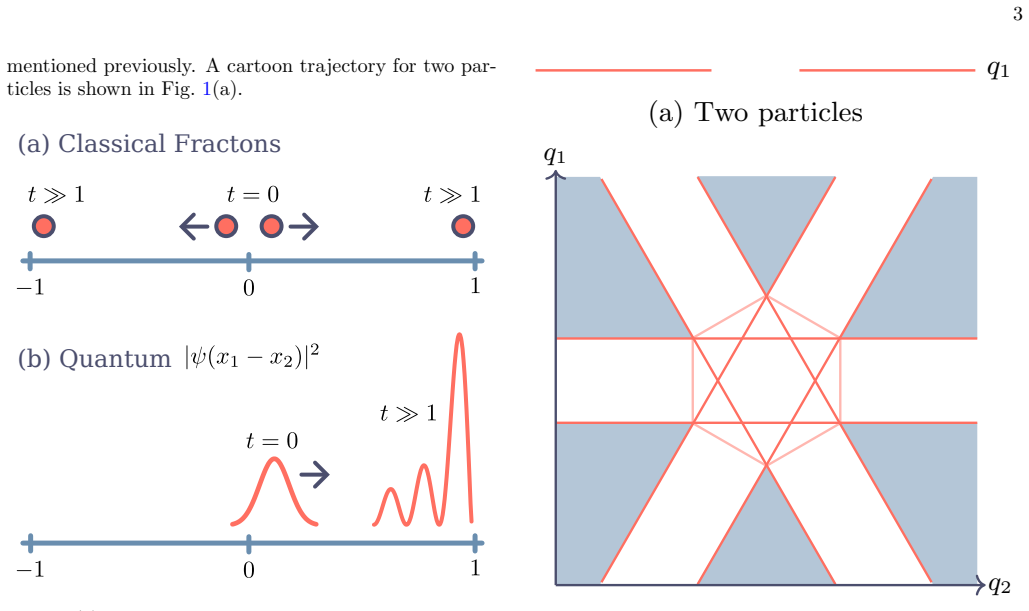
Semiclassical intuition from the freezing time To understand the spectral transition of Eq. (11), let us begin with a review of the classical trajectories of two fractons. A two-body trajectory is shown in Fig. 1(a). We see that generically two closely separated particles (nec...
-
[10]
The importance of this condition stems from the spectral theorem, which guarantees that a self-adjoint operator has a real spectrum and a complete set of eigen- functions
Self-adjointness For a quantum Hamiltonian to represent a physical ob- servable, it must be a self-adjoint operator on a Hilbert space—in our case, the space of square-integrable func- tionsL 2([−1,1]) defined on the coordinate spacex∈ [−1,1]. The importance of this condition ...
-
[11]
This implies [19] that the self-adjoint extensions are parameterized by a 2×2 unitary matrix, or four real parameters
Self-adjoint boundary conditions For the limit-circle case (θ <2), the deficiency indices of ˆHare (n +, n−) = (2,2), since for any non-real energy E, the equation ˆHψ=Eψhas two square-integrable solutions on [−1,1]. This implies [19] that the self-adjoint extensions are param...
-
[12]
We takeK= 1−x 2, which vanishes linearly atx=±1
Exactly solvable case Forθ= 1, where we expect a discrete spectrum, we can exactly solve the Schr¨ odinger equation. We takeK= 1−x 2, which vanishes linearly atx=±1. WritingE l = l(l+ 1), we have (1−x 2)ψ′′ −2xψ ′ +l(l+ 1)ψ= 0,(20) which is exactly the Legendre differential eq...
-
[13]
The existence of a spectral transition atθ= 2
-
[14]
The pile up of probability at the edges forθ >2, and standard boundary reflection forθ <2
-
[15]
Spectrum transition Marvelously, we havea∝τ f defined in Eq. (14), and therefore asθis tuned acrossθ= 2, the domain in which the Schr¨ odinger operator is defined changes from a finite interval where we can expect a discrete spectrum, to an infinite interval where we can expec...
-
[16]
internal line
Dynamics The energy spectrum transitions from a discrete one to a continuous one as we crossθ= 2. How does the dynamics change as this transition is crossed? Once again we use the Liouville transform to tackle this problem, as the dynamics of an ordinary particle is easy to so...
2020
-
[17]
=e iθg ψ(q1, q2) (C7) Doublets:ψ a(q′ 1, q′
-
[18]
=w(g) abψb(q1, q2),(C8) The various possibilities forθ g andw g are listed in Ta- ble I, up to a basis choice. Appendix D: Continuum formulation Recall that when one passes from first to second quan- tization, we make the following replacements for one bodyA i and two bodyB ij...
-
[19]
R. M. Nandkishore and M. Hermele, Fractons, Annual Review of Condensed Matter Physics10, 295 (2019), https://doi.org/10.1146/annurev-conmatphys-031218- 18 013604
2019 doi
-
[20]
Pretko, X
M. Pretko, X. Chen, and Y. You, Fracton phases of matter, International Journal of Modern Physics A35, 2030003 (2020)
2020
-
[21]
Gromov and L
A. Gromov and L. Radzihovsky, Fracton matter (2022), arXiv:2211.05130 [cond-mat.str-el]
2022 arXiv
-
[22]
Chamon, Quantum glassiness in strongly correlated clean systems: An example of topological overprotection, Phys
C. Chamon, Quantum glassiness in strongly correlated clean systems: An example of topological overprotection, Phys. Rev. Lett.94, 040402 (2005)
2005
-
[23]
Haah, Local stabilizer codes in three dimensions with- out string logical operators, Phys
J. Haah, Local stabilizer codes in three dimensions with- out string logical operators, Phys. Rev. A83, 042330 (2011)
2011
-
[24]
Vijay, J
S. Vijay, J. Haah, and L. Fu, Fracton topological order, generalized lattice gauge theory, and duality, Phys. Rev. B94, 235157 (2016)
2016
-
[25]
Gorantla, H
P. Gorantla, H. T. Lam, N. Seiberg, and S.-H. Shao, Low- energy limit of some exotic lattice theories and uv/ir mix- ing, Phys. Rev. B104, 235116 (2021)
2021
-
[26]
You and R
Y. You and R. Moessner, Fractonic plaquette-dimer liq- uid beyond renormalization, Phys. Rev. B106, 115145 (2022)
2022
-
[27]
Khemani, M
V. Khemani, M. Hermele, and R. Nandkishore, Local- ization from hilbert space shattering: From theory to physical realizations, Phys. Rev. B101, 174204 (2020)
2020
-
[28]
P. Sala, T. Rakovszky, R. Verresen, M. Knap, and F. Poll- mann, Ergodicity breaking arising from hilbert space fragmentation in dipole-conserving hamiltonians, Phys. Rev. X10, 011047 (2020)
2020
-
[29]
Prakash, A
A. Prakash, A. Goriely, and S. Sondhi, Classical nonrel- ativistic fractons, Phys. Rev. B109, 054313 (2024)
2024
-
[30]
Prakash, Y
A. Prakash, Y. Sadki, and S. Sondhi, Machian frac- tons, hamiltonian attractors, and nonequilibrium steady states, Physical Review B110, 024305 (2024)
2024
-
[31]
Babbar, Y
A. Babbar, Y. Sadki, A. Prakash, and S. Sondhi, Classical fractons: Local chaos, global broken ergodicity, and an arrow of time, Physical Review B111, 245134 (2025)
2025
-
[32]
Sadki, A
Y. Sadki, A. Prakash, S. L. Sondhi, and D. P. Arovas, Phase space fractons (2025), arXiv:2502.02650 [cond- mat.stat-mech]
2025
-
[33]
In the quantum case, however, the operators ˆqN and ˆπN do not commute, satisfying [ˆqN ,ˆπN ] =i
In the classical case, one can simply fix the center-of- mass positionq N and momentumπ N to definite values. In the quantum case, however, the operators ˆqN and ˆπN do not commute, satisfying [ˆqN ,ˆπN ] =i. Their values are therefore subject to the uncertainty principle and ...
-
[34]
Zettl,Sturm-Liouville Theory, 121 (American Mathe- matical Soc., 2005)
A. Zettl,Sturm-Liouville Theory, 121 (American Mathe- matical Soc., 2005)
2005
-
[35]
L. L. Littlejohn and A. Zettl, The legendre equation and its self-adjoint operators, Electronic Journal of Differen- tial Equations2011, 1 (2011)
2011
-
[36]
C. A. Stuart, Stability analysis for a family of degenerate semilinear parabolic problems., Discrete & Continuous Dynamical Systems: Series A38(2018)
2018
-
[37]
Reed and B
M. Reed and B. Simon,Methods of modern mathematical physics, Vol. 1 (Academic press New York, 1972)
1972
-
[38]
Hille,Lectures on Ordinary Differential Equations (Addison-Wesley, 1969)
E. Hille,Lectures on Ordinary Differential Equations (Addison-Wesley, 1969)
1969
-
[39]
Atkinson, Wave propagation and the bremmer series, Journal of mathematical analysis and applications1, 255 (1960)
F. Atkinson, Wave propagation and the bremmer series, Journal of mathematical analysis and applications1, 255 (1960)
1960
-
[40]
Heading,An introduction to phase-integral methods (Courier Corporation, 2013)
J. Heading,An introduction to phase-integral methods (Courier Corporation, 2013)
2013
-
[41]
M. V. Berry and K. Mount, Semiclassical approximations in wave mechanics, Reports on Progress in Physics35, 315 (1972)
1972
-
[42]
Physically, each integral corresponds to a point where the wave reflects
Generally speaking, we must iterate this proce- dure, each time picking up an additional integral:´ dξ1 ´ dξ2 · · · ´ dξn, and so on. Physically, each integral corresponds to a point where the wave reflects
-
[43]
Moessner and J
R. Moessner and J. T. Chalker, Properties of a classical spin liquid: The heisenberg pyrochlore antiferromagnet, Phys. Rev. Lett.80, 2929 (1998)
1998
-
[44]
J. T. Chalker, Geometrically frustrated antiferromagnets: Statistical mechanics and dynamics, inIntroduction to Frustrated Magnetism: Materials, Experiments, Theory (Springer Berlin Heidelberg, Berlin, Heidelberg, 2011) pp. 3–22
2011
-
[45]
Shender, Antiferromagnetic garnets with fluctuation- ally interacting sublattices, Soviet Journal of Experimen- tal and Theoretical Physics56, 178 (1982)
E. Shender, Antiferromagnetic garnets with fluctuation- ally interacting sublattices, Soviet Journal of Experimen- tal and Theoretical Physics56, 178 (1982)
1982
-
[46]
C. L. Henley, Ordering by disorder: Ground-state selec- tion in fcc vector antiferromagnets, Journal of Applied Physics61, 3962 (1987)
1987
-
[47]
Morningstar, V
A. Morningstar, V. Khemani, and D. A. Huse, Kinetically constrained freezing transition in a dipole-conserving sys- tem, Phys. Rev. B101, 214205 (2020)
2020
-
[48]
Pozderac, S
C. Pozderac, S. Speck, X. Feng, D. A. Huse, and B. Skin- ner, Exact solution for the filling-induced thermalization transition in a one-dimensional fracton system, Phys. Rev. B107, 045137 (2023)
2023
-
[49]
Classen-Howes, R
J. Classen-Howes, R. Senese, and A. Prakash, Univer- sal freezing transitions of dipole-conserving chains, Phys. Rev. B112, 125148 (2025)
2025
-
[50]
Pretko, The fracton gauge principle, Phys
M. Pretko, The fracton gauge principle, Phys. Rev. B98, 115134 (2018)
2018
-
[51]
A. L. Fetter and J. D. Walecka,Quantum theory of many- particle systems(Courier Corporation, 2012)
2012
-
[52]
Gromov, Towards classification of fracton phases: The multipole algebra, Phys
A. Gromov, Towards classification of fracton phases: The multipole algebra, Phys. Rev. X9, 031035 (2019)
2019
-
[53]
Gromov, A
A. Gromov, A. Lucas, and R. M. Nandkishore, Fracton hydrodynamics, Phys. Rev. Res.2, 033124 (2020)
2020
Reviewed August 4, 2026 · model on record in the stance chip above.
Discussion (0). Sign in to comment.