REVIEW 2 major objections 2 minor 1 cited by
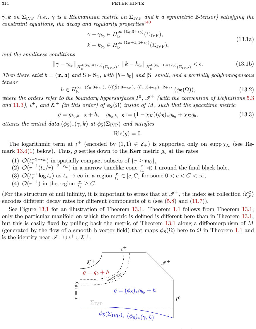
Spacetimes from initial data near subextremal Kerr black holes settle to a nearby Kerr solution at rate O(t_*^{-2-ε_K}) in spatially compact regions.
Reviewed by Pith at T0; open to challenge. T0 means a machine referee read the full paper against a public rubric. the ladder, T0–T4 →
T0 review · grok-4.3
2026-06-29 02:52 UTC pith:4EXB32UR
load-bearing objection Hintz claims to settle nonlinear stability for the full subextremal Kerr family, but the argument treats two same-author companion papers as black boxes for the key damping and estimate inputs. the 2 major comments →
Nonlinear stability of subextremal Kerr black holes
The pith
A machine-rendered reading of the paper's core claim, the machinery that carries it, and where it could break.
Core claim
We settle the global nonlinear stability problem for the family of Kerr black holes in the full subextremal range: spacetimes evolving from initial data close to those of a subextremal Kerr black hole as solutions of the Einstein vacuum equation Ric(g)=0 settle down to a nearby member of the Kerr family at the rate O(t_*^{-2-ε_K}) in spatially compact regions. For the initial data we require O(r^{-1-ε0})-decay for ε0>0, more precisely an arbitrary but finite expansion into terms r^{-z}(log r)^k where z>1, k in N_0, plus a remainder with O(r^{-3-ε0})-decay. The gauge source terms, final black hole parameters, and gravitational wave tail are treated as unknowns in the nonlinear iteration.
What carries the argument
Generalized wave map gauge modified by gauge source terms lying in a finite-dimensional space determined by the initial-data expansion, inside a nonlinear Nash-Moser iteration scheme that solves the gauge-fixed Einstein equation directly.
Load-bearing premise
The two companion papers supply a strong form of constraint damping valid throughout the subextremal range together with tame estimates for the relevant linearized wave equations.
What would settle it
An explicit initial-data set with the stated decay whose evolution under Ric(g)=0 either fails to approach any Kerr solution or decays slower than O(t_*^{-2-ε_K}) in a fixed compact region.
If this is right
- The final mass and angular momentum are recovered as part of the solution rather than prescribed in advance.
- The same gauge and iteration framework controls the gravitational wave tail at the stated rate.
- The argument applies to initial data whose expansion may contain arbitrarily many logarithmic terms.
- No reduction of the Einstein equation to scalar wave equations is required except for the linear mode-stability step.
Where Pith is reading between the lines
- The decay rate O(t_*^{-2-ε}) is slow enough that late-time tails remain visible in spatially compact observations but fast enough to guarantee asymptotic flatness at future null infinity.
- The method separates the determination of the final Kerr parameters from the dynamical decay, which may allow similar iteration schemes when matter fields or cosmological constants are added.
- Numerical evolutions of near-Kerr data could directly measure the predicted power-law index in the approach to stationarity.
Editorial analysis
A structured set of objections, weighed in public.
Referee Report
Summary. The manuscript claims to prove the global nonlinear stability of subextremal Kerr black holes for the Einstein vacuum equations. Initial data close to a subextremal Kerr solution (with O(r^{-1-ε_0}) decay, including finite expansions in r^{-z}(log r)^k for z>1) evolve to a nearby Kerr black hole, with decay O(t_*^{-2-ε_K}) in spatially compact regions. The proof uses a generalized wave map gauge with finite-dimensional gauge source terms (treated as unknowns), a Nash-Moser iteration scheme, and works directly with the tensorial equation (except for Teukolsky reduction in linear mode stability). The argument relies on two companion papers for constraint damping and tame estimates.
Significance. If established, the result would be a significant contribution to mathematical general relativity by resolving nonlinear stability for the full subextremal Kerr family. The direct tensorial approach and incorporation of gauge source terms and final parameters into the nonlinear iteration are strengths. The paper also notes the use of mode stability via the Teukolsky equation.
major comments (2)
- [Abstract, paragraph on reliance on companion papers] Abstract, paragraph on reliance on companion papers: the nonlinear iteration scheme and the claimed O(t_*^{-2-ε_K}) decay in compact regions are obtained by bootstrapping from the tame estimates (with weak decay) supplied by the second companion paper, while solving for gauge source terms and Kerr parameters; these estimates are asserted to cover the linearizations of the gauge-fixed Einstein equation, but no verification or closure check under the nonlinear iteration is provided here.
- [Abstract, paragraph on reliance on companion papers] Abstract, paragraph on reliance on companion papers: the formulation of the gauge-fixed Einstein equation uses a strong form of constraint damping valid throughout the subextremal range |a|<M as a black box from the first companion paper; if this damping does not suppress violations at the required rate near extremality, the global stability statement does not follow.
minor comments (2)
- [Abstract] Abstract: the decay rate notation O(t_*^{-2-ε_K}) and the parameter ε_K are not defined in the abstract; a parenthetical clarification would improve readability.
- [Abstract] Abstract: the initial data expansion is stated as arbitrary but finite into r^{-z}(log r)^k with z>1; specifying the admissible range of z and k explicitly would aid precision.
Simulated Author's Rebuttal
We thank the referee for their detailed reading of the manuscript. We address the two major comments point by point below.
read point-by-point responses
-
Referee: [Abstract, paragraph on reliance on companion papers] Abstract, paragraph on reliance on companion papers: the nonlinear iteration scheme and the claimed O(t_*^{-2-ε_K}) decay in compact regions are obtained by bootstrapping from the tame estimates (with weak decay) supplied by the second companion paper, while solving for gauge source terms and Kerr parameters; these estimates are asserted to cover the linearizations of the gauge-fixed Einstein equation, but no verification or closure check under the nonlinear iteration is provided here.
Authors: The manuscript states in the abstract and develops in the main text that the linearizations arising at each step of the Nash-Moser iteration belong to the general class of wave-type equations for which the second companion paper supplies tame estimates. The iteration is constructed precisely so that the gauge source terms and final Kerr parameters remain within the finite-dimensional spaces for which the estimates close; the weak decay supplied by the companion is then upgraded to the stated O(t_*^{-2-ε_K}) rate by the asymptotic analysis performed here. A more explicit sentence summarizing this closure can be added to the abstract or introduction for clarity. revision: partial
-
Referee: [Abstract, paragraph on reliance on companion papers] Abstract, paragraph on reliance on companion papers: the formulation of the gauge-fixed Einstein equation uses a strong form of constraint damping valid throughout the subextremal range |a|<M as a black box from the first companion paper; if this damping does not suppress violations at the required rate near extremality, the global stability statement does not follow.
Authors: The first companion paper establishes the strong constraint damping for the full subextremal range |a|<M, including the decay rates needed to control violations near extremality. The present work invokes this result as a black box exactly as described, and the global stability statement therefore inherits the range and rates proved in the companion. No additional verification is required in this manuscript beyond the statement already given. revision: no
Circularity Check
Central nonlinear stability result depends on black-box self-citations for constraint damping and tame estimates
specific steps
-
self citation load bearing
[abstract]
"This paper relies on two companion papers by the author. The first one introduces a strong form of constraint damping in the full subextremal range, which we use in our formulation of the gauge-fixed Einstein equation as a black box. The second one provides tame estimates (albeit with weak decay) for forward solutions of a general class of wave-type equations, which we show here to include the linearizations of the gauge-fixed Einstein equation arising in our nonlinear iteration scheme; these estimates are the starting point for our detailed asymptotic analysis."
The nonlinear iteration scheme and the claimed decay rate are obtained only after bootstrapping from the weak-decay tame estimates while solving for gauge source terms and final Kerr parameters. Both the damping and the tame estimates are supplied exclusively by the two self-cited companion papers and are invoked as black boxes; the stability statement therefore does not follow without those prior self-citations.
full rationale
The paper's derivation of the O(t_*^{-2-ε_K}) decay for subextremal Kerr stability proceeds via a Nash-Moser iteration on the gauge-fixed Einstein equation. This iteration is explicitly constructed to take as black-box inputs (1) strong constraint damping valid for |a|<M and (2) tame estimates for the relevant linearized wave equations; both are supplied by two companion papers by the same author. The abstract states that these are used directly without further derivation here, and the asymptotic analysis bootstraps from the weak-decay tame estimates. No external benchmarks, machine-checked verification, or independent falsifiability of the companions is provided in this manuscript, so the central claim reduces to the self-citation chain.
Axiom & Free-Parameter Ledger
axioms (2)
- domain assumption Linear mode stability via reduction to the Teukolsky equation holds in the subextremal range
- domain assumption The generalized wave map gauge with finite-dimensional source terms yields a well-posed gauge-fixed Einstein equation
Cite this review
Pith. "Pith review of Nonlinear stability of subextremal Kerr black holes." pith.science (2026). https://pith.science/paper/4EXB32UR
@misc{pith2026260628253,
  author       = {Pith},
  title        = {Pith review of: Nonlinear stability of subextremal Kerr black holes},
  year         = {2026},
  howpublished = {\url{https://pith.science/paper/4EXB32UR}},
  note         = {Machine review of arXiv:2606.28253}
}
read the original abstract
We settle the global nonlinear stability problem for the family of Kerr black holes in the full subextremal range: spacetimes evolving from initial data close to those of a subextremal Kerr black hole as solutions of the Einstein vacuum equation ${\rm Ric}(g)=0$ settle down to a nearby member of the Kerr family at the rate $\mathcal{O}(t_*^{-2-\epsilon_{\mathcal K}})$ in spatially compact regions. For the initial data, we require $\mathcal{O}(r^{-1-\epsilon_0})$-decay for $\epsilon_0>0$ -- more precisely, an arbitrary but finite expansion into terms $r^{-z}(\log r)^k$ where $z>1$, $k\in\mathbb{N}_0$, plus a remainder term with $\mathcal{O}(r^{-3-\epsilon_0})$-decay. We use a generalized wave map gauge modified using gauge source terms that lie in a suitable finite-dimensional space determined by the expansion of the initial data. Like the final black hole parameters (mass and angular momentum) and the gravitational wave tail, the gauge source terms are treated as unknowns in a nonlinear (Nash-Moser) iteration scheme. We work directly with the tensorial equation and in particular do not rely on reductions to scalar equations (except insofar as a reduction to the Teukolsky equation is used in the proof of linear mode stability). This paper relies on two companion papers by the author. The first one introduces a strong form of constraint damping in the full subextremal range, which we use in our formulation of the gauge-fixed Einstein equation as a black box. The second one provides tame estimates (albeit with weak decay) for forward solutions of a general class of wave-type equations, which we show here to include the linearizations of the gauge-fixed Einstein equation arising in our nonlinear iteration scheme; these estimates are the starting point for our detailed asymptotic analysis.
Figures
Forward citations
Cited by 1 Pith paper
-
A Physical space derivation of Morawetz-Energy estimates in Kerr spacetimes with large angular momentum
Physical-space Morawetz-energy estimates hold for the scalar wave equation on Kerr with |a|/m ≤ 0.75, via trapping-set characterization, Stogin-type low-frequency control, and a physical-space Whiting transform.
discussion (0)
Sign in with ORCID, Apple, or X to comment. Anyone can read and Pith papers without signing in.