REVIEW 4 major objections 3 minor 73 references
Curvature acts as a position-dependent mass for virtual particles, shifting cavity frequencies in a way geometric optics cannot.
Reviewed by Pith at T0; open to challenge. T0 means a machine referee read the full paper against a public rubric. the ladder, T0–T4 →
T0 review · deepseek-v4-flash
2026-08-03 18:07 UTC pith:DMYLAQGM
load-bearing objection Novel idea—curvature as a local mass shift in vacuum loops—but the central calculation is invalid: the 4D loop integral is truncated to 3D, turning a log-divergence into a finite coefficient. the 4 major comments →
Geometry-Induced Vacuum Polarization and Mode Shifts in Maxwell-Klein-Gordon Theory
The pith
A machine-rendered reading of the paper's core claim, the machinery that carries it, and where it could break.
Core claim
The central claim is that the geometric potential Sigma_geom(r) — assembled from mean curvature, the second fundamental form, and ambient Ricci curvature — is not merely a kinematic potential for single particles but a locally varying mass term for virtual fluctuations. The one-loop photon self-energy acquires a curvature correction delta_Pi_T proportional to Sigma_geom with the universal low-frequency coefficient I0 = 3q^2/(8 pi m). In the long-wavelength limit (|Q|R << 1) the relative mode shift becomes Delta_omega_n/omega_n = I0/(2 epsilon_0 omega^2 U_n) integral d^3r |E_n|^2 Sigma_geom, so curvature acts as a local renormalization environment: the response is finite, gauge-invariant, and
What carries the argument
The central object is the geometric potential Sigma_geom = 1/4 ||H||^2 - 1/2 ||II||^2 - 1/2 sum_a Ric_M(nu_a, nu_a), a combination of embedding invariants; in flat space it collapses to -1/4 (kappa_1 - kappa_2)^2, so it is purely a measure of curvature anisotropy. It enters through the scalar resolvent G_Sigma = [-nabla^2 - omega^2 + m^2 + Sigma_geom]^{-1}, converting curvature into a position-dependent mass that virtual particles experience. The carrying identity is the loop coefficient I0(0;m) = 3q^2/(8 pi m), which converts the spatial average of Sigma_geom into a frequency shift via the master formula Eq. (19).
Load-bearing premise
The result stands only if the four-dimensional vacuum loop can be reduced to a three-dimensional spatial integral whose value happens to be finite; if the omitted energy integration is performed in full 4D, the coefficient I0 would diverge and the claimed finite, scheme-independent shift disappears.
What would settle it
Compute Eq. (A1) in full four-dimensional Euclidean space with a UV cutoff Lambda, without truncating the k0 integration. If the transverse part I0(Lambda,m) depends on Lambda (e.g., grows as log Lambda) instead of equaling the constant 3q^2/(8 pi m), the central prediction of a finite, geometry-induced mode shift is refuted; equivalently, in dimensional regularization with d=4-2 epsilon, any residual 1/epsilon pole in delta_Pi_T would disprove the claim.
If this is right
- Modes whose electric energy concentrates where curvature is most anisotropic experience the largest shift; for a Gaussian bump, higher-order radial modes that sample the potential's peak at rho ~ sqrt(2) sigma shift more than the fundamental mode.
- An infinite cylindrical shell of radius R exhibits a universal redshift Delta_omega/omega proportional to -1/(4 R^2), independent of the mode profile along the axis.
- A torus breaks poloidal symmetry: the shift acquires an angular dependence 1 - 2 epsilon <cos theta |E|^2>/<|E|^2>, so modes on the inner equator shift more than those on the outer equator.
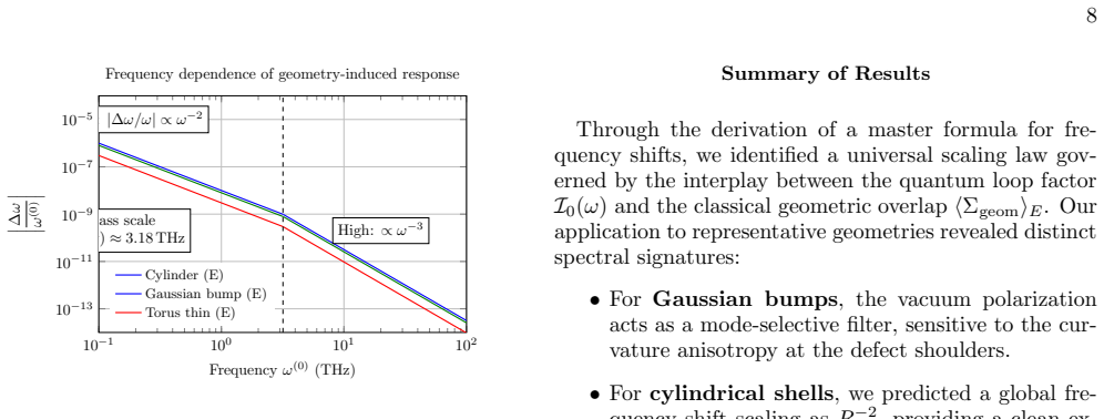
- The frequency dependence is universal: subgap modes shift as omega^{-2}, while high-frequency modes shift as omega^{-3}, preserving causality via the Kramers-Kronig relations.
- The ambient space contributes a constant offset: in a CP^1 ambient manifold the potential gains an extra -1/r_0^2 term, shifting all modes uniformly and providing a spectral signature of compactified dimensions.
Where Pith is reading between the lines
- Because the same geometric potential appears in the single-particle effective equation, the loop-level mechanism should apply to any charged quasiparticle confined to a curved layer; a natural extension is to Dirac materials, where curvature and pseudomagnetic fields coexist, and the predicted shift could be compared with strained-graphene resonators.
- The formalism implies a local, curvature-dependent refractive index; a direct probe would be measuring group delay in plasmonic waveguides wrapped around cylinders or tori, where the delay should vary with the local curvature overlap even at fixed path length.
- The paper's quasi-3D truncation of the loop integral (dropping the energy integration) is the step that makes I0 finite; a full 4D evaluation would likely introduce a cutoff dependence set by the layer thickness h, which would change the predicted scaling and offer a way to distinguish this mechanism from bulk Casimir-like effects.
Editorial analysis
A structured set of objections, weighed in public.
Referee Report
Summary. The paper considers a Maxwell–Klein–Gordon system in a (3+1)-dimensional bulk, with a scalar field subject to geometric confinement. It assumes that the thin-layer geometric potential Σ_geom(r) acts as a position-dependent mass term M^2(r)=m^2+Σ_geom(r) in the bulk Lagrangian. The authors compute the one-loop photon self-energy to first order in Σ_geom and claim that, in the long-wavelength limit, the resulting transverse polarization yields a finite, gauge-invariant frequency shift proportional to the electric-energy-weighted average of Σ_geom (Eq. 19). Applications to Gaussian bumps, cylinders, and tori give predicted mode shifts, and numerical estimates are presented for high-Q cavities and plasmonic systems.
Significance. If established, the result would provide a new mechanism by which extrinsic and ambient curvature modifies quantum vacuum fluctuations, with potentially measurable spectroscopic signatures. The paper is clearly organized, and the applications are straightforward once the master formula is accepted; the derivation from the assumed model is transparent and yields explicit falsifiable predictions. However, the central loop calculation is flawed, and the purported finite shift is an artifact of a dimensional truncation. The paper also assumes rather than derives the mass-correction hypothesis. Thus the current manuscript does not make a reliable contribution.
major comments (4)
- [Appendix A, Eqs. (A1)–(A2)] The reduction of the 4D loop to a 3D integral is invalid. Performing the Euclidean k0_E integration in (A1) at Ω=0 yields a denominator power (|k|^2+m^2)^{-5/2} and a remaining spatial integrand ~ |k|^2/(|k|^2+m^2)^{5/2} d^3k, which is logarithmically divergent. Eq. (A2) instead uses (|k|^2+m^2)^{-3} with d^3k, which is UV finite. The finite value I0=3q^2/(8πm) is therefore an artifact of a 3D truncation. Since I0 multiplies every curvature invariant in Eqs. (15)–(19) and the numerical estimates of Section III.F, the central claim of a finite, scheme-independent shift is unsupported.
- [Section II, Dimensionality, Regularization, and Renormalization] The text states that the single-mass-insertion diagram is logarithmically divergent in D=4, then immediately claims that after integrating out k0 the remaining spatial integral is finite. This is internally contradictory. Moreover, the gauge-invariant transverse projection does not remove the divergence of the photon self-energy; in scalar QED the transverse part is precisely the quantity requiring charge renormalization. The claimed DimReg 'finite part' is therefore scheme-dependent, not a universal geometric shift.
- [Section II, Eq. (7)] The one-loop photon self-energy of scalar QED contains, in addition to the double-derivative bubble, a seagull (contact) term proportional to g_μν GΣ(x,x) arising from the q^2 A^2 |φ|^2 vertex. Eq. (7) as written omits this term. Without it, the expression is not transverse, and the decomposition (11) into δΠ_T is not justified. The statement 'preserves transversality by the Ward identity' is therefore not supported by the displayed formulas.
- [Section I and Section II, Eqs. (1)–(3)] The identification M^2(r)=m^2+Σ_geom(r) is introduced as a 'central hypothesis' and is used to write the bulk Lagrangian. No derivation is given from the constrained/thin-layer quantum field theory; the claim that real modes see a 2D surface while virtual fluctuations probe the 3D volume is asserted. Consequently, the conclusions state 'we have established' a result whose physical premise remains an assumption. This is a limitation of the paper's claim, not merely a presentation issue.
minor comments (3)
- [Eq. (12)] The phrase 'overlines denote local values in the gradient expansion' is vague; the definitions of the averaged field Σ_geom(0) and the momentum variables Q_i should be spelled out.
- [Eq. (32)] The torus shift is given to first order in ϵ. Since Eq. (31) contains an ϵ^2 term, check whether this term contributes at the same order after angular averaging for modes localized on the inner or outer equator.
- [Section III.F] The numerical estimate Δω/ω ~ 10^-4–10^-3 for m*=0.01m_e and R=50 nm appears larger than the stated α_eff (λ_c/R)^2 scaling would suggest; please provide the numerical details and justify the enhancement factor.
Circularity Check
The 'geometry-induced running' is the assumed M² = m² + Σ_geom ansatz read back through a linear-response loop; the finite prefactor I0 is also fixed by a non-equivalent 3D truncation of the 4D integral.
specific steps
-
self definitional
[Eq. (1) and Eqs. (15)-(19), Section II]
"L = −1/4 FμνFμν + (Dμϕ)∗(Dμϕ) − (m² + Σgeom(r)) |ϕ|² ... δΠT(Ω;Q→0) = (1/4 ||H||² − 1/2 ||II||² − 1/2 Σ_a Ric_M(ν_a,ν_a)) I0(Ω;m) + O(∇²Σgeom)"
The action already contains the proposed effect: Eq. (1) defines the scalar mass as m² + Σ_geom(r). The one-loop calculation then returns exactly the same Σ_geom bracket in Eq. (15), multiplied by I0, and Eq. (19) turns it into the predicted frequency shift. Thus the central claim that curvature enters the vacuum as a position-dependent mass correction is not derived from independent dynamics; it is placed in the Lagrangian as the starting ansatz and read back out through a linear-response calculation.
-
other
[Appendix A, Eqs. (A1)-(A2); Section II 'Dimensionality, Regularization']
"Integrating out the temporal component ∫ dk0_E effectively yields a spatial loop factor. For the specific projection relevant to the transverse susceptibility (Eq. (13)), the integral reduces to a 3D momentum integration: I0(0;m) = q² ∫ d³k/(2π)³ 4k²/(k² + m²)³."
The advertised finite gauge-invariant coefficient is imposed by this step rather than obtained from the D=4 loop. Performing the k0_E integral in Eq. (A1) at Ω=0 gives ∫ dk0_E (k0_E² + k² + m²)^{-3} ∝ (k² + m²)^{-5/2}; the remaining ∫ d³k k²/(k²+m²)^{5/2} is logarithmically divergent. The convergent 3D form used here, with denominator (k²+m²)^{-3}, is not equivalent to the starting integral. The constant I0 = 3q²/(8πm) multiplying every curvature invariant is therefore an artifact of the chosen 3D truncation, not a computed finite part.
full rationale
The paper's central observable, Eq. (19), is a genuine linear-response consequence of the Lagrangian (1), so the arithmetic from action to frequency shift is self-contained; however the crucial physical input—M²(r)=m²+Σ_geom(r)—is explicitly assumed ('our central hypothesis'), and the only universal coefficient I0 is obtained by replacing the 4D loop integral by a convergent 3D integral. I treat the Appendix A issue as a constructive reduction of the numerical claim rather than a fit to data, so it raises the circularity score, but the headline concern is better classified as a severe computational/regularization defect. The self-citation to Ref. [16] for Σ_geom is standard and externally supported by the da Costa line of results, so I do not count it as load-bearing circularity. Overall: one definitional ansatz readout plus one constructed loop coefficient yield partial circularity, score 4.
Axiom & Free-Parameter Ledger
axioms (3)
- ad hoc to paper The geometric potential Σ_geom(r) from thin-layer quantization acts as a local mass correction in the bulk Lagrangian: M^2(r) = m^2 + Σ_geom(r).
- ad hoc to paper The one-loop vacuum polarization loop integral may be reduced to a 3D spatial integral (spatial loop momentum k only, denominator (k^2 + m^2 - Ω^2)^3).
- domain assumption The flat-space vacuum polarization is renormalized on-shell (Π(0)=0), while the geometry-induced part is UV finite without additional counterterms.
read the original abstract
Geometric confinement is known to modify single-particle dynamics through effective potentials, yet its imprint on the interacting quantum vacuum remains largely unexplored. In this work, we investigate the Maxwell--Klein--Gordon system constrained to curved surfaces and demonstrate that the geometric potential $\Sigma_{\mathrm{geom}}(\mathbf{r})$ acts as a local renormalization environment. We show that extrinsic curvature modifies the scalar loop spectrum, entering the vacuum polarization as a position-dependent mass correction $M^2(\mathbf{r}) \to m^2 + \Sigma_{\mathrm{geom}}(\mathbf{r})$. This induces a finite, gauge-invariant ``geometry-induced running'' of the electromagnetic response. In the long-wavelength regime ($|{\bf Q}|R \ll 1$), we derive a closed-form expression for the relative frequency shift $\Delta\omega/\omega$, governed by the overlap between the electric energy density and the geometric potential. Applying this formalism to Gaussian bumps, cylindrical shells, and tori, we identify distinct spectral signatures that distinguish these quantum loop corrections from classical geometric optics. Our results suggest that spatial curvature can serve as a tunable knob for ``vacuum engineering,'' offering measurable shifts in high-$Q$ cavities and plasmonic systems.
Figures


Reference graph
Works this paper leans on
-
[1]
for intermediate field-theoretic derivations to main- tain notational clarity. However, to facilitate comparison with spectroscopic measurements, we explicitly restore SI units (including the vacuum permittivityε 0) in the final expressions for susceptibilities and frequency shifts. Scalar resolvent and local expansions Introduce the static-frequency scal...
-
[2]
(21) Two immediate consequences follow
=− 1 4 (κ1 −κ 2)2 ≤0. (21) Two immediate consequences follow. First, near-umbilic surfaces (κ 1 ≈κ 2) yield a weak geometric potential and hence smaller shifts. Second, highly anisotropic curva- ture (|κ 1 −κ 2|large), as near saddle-like regions, en- hances|Σ geom|and typically increases the magnitude of the susceptibility correction in Eq. (18), leading...
-
[3]
0 𝜋 2𝜋 −15 −10 −5 0 𝑋=𝑘𝑥 ˜Σ(𝑋) ˜Σ𝐸(𝑋)=−cos 2 𝑋 ˜ΣCP1 (𝑋)=−cos 2 𝑋− 4 𝑎2 𝑘4𝑟 2 FIG
Geometric Potential Construction The radial curvatureκ ρ and azimuthal curvatureκ ϕ are approximated by: κρ ≈∂ 2 ρz=− h σ2 1− ρ2 σ2 e−ρ2/2σ2 ,(24) κϕ ≈ 1 ρ ∂ρz=− h σ2 e−ρ2/2σ2 .(25) The Euclidean geometric potential is proportional to the square of their difference (the anisotropy): Σbump geom (ρ) =− 1 4 (κρ −κ ϕ)2 =− h2 4σ4 ρ σ 4 e−ρ2/σ2 .(26) This poten...
-
[4]
(26) into the master formula, the rel- ative frequency shift is: ∆ω ω =− I0(ω;m) 2ε0ω2 FE h2 4σ4 Cb,(27) whereC b =⟨(ρ/σ) 4e−ρ2/σ2 ⟩E is the modal overlap factor
Frequency Shift and Mode Selectivity Substituting Eq. (26) into the master formula, the rel- ative frequency shift is: ∆ω ω =− I0(ω;m) 2ε0ω2 FE h2 4σ4 Cb,(27) whereC b =⟨(ρ/σ) 4e−ρ2/σ2 ⟩E is the modal overlap factor. Physics Discussion:The factor (ρ/σ) 4 introduces a strongspatial filtering effect. •For fundamental modes (Gaussian-like) centered at ρ= 0, ...
-
[5]
Potential and Shift The principal curvatures areκ 1 = 1/R(azimuthal) andκ 2 = 0 (axial). The Euclidean geometric potential is constant: Σcyl geom =− 1 4 1 R −0 2 =− 1 4R2 .(28) The frequency shift becomes simply: ∆ω ω cyl =− I0(ω;m) 2ε0ω2 FE 1 4R2 .(29) This represents aredshiftof the mode frequencies pro- portional to the inverse square of the radius
-
[6]
3, the vac- uum polarization pattern is uniform, but the magnitude is renormalized by the ambient background
Comparison withCP 1 Ambient If the cylinder is embedded inCP 1, the potential ac- quires the ambient term: Σtotal =− 1 4R2 − 1 r2 0 .(30) As illustrated in the 3D visualization of Fig. 3, the vac- uum polarization pattern is uniform, but the magnitude is renormalized by the ambient background. The quanti- tative scaling behavior is further detailed in Fig...
-
[7]
Unlike the cylinder, this potential de- pends explicitly on the poloidal angleθ
Thin-Torus Expansion In the thin-torus limit (a≪R), the geometric poten- tial is: Σtor geom(θ)≈ − 1 4a2 1−2ϵcosθ+ϵ 2 cos2 θ ,(31) whereϵ=a/R. Unlike the cylinder, this potential de- pends explicitly on the poloidal angleθ
-
[8]
Thisθ-dependence breaks the symmetry between inner and outer distinct modes
Poloidal Mode Dependence The frequency shift depends on the mode asymmetry: ∆ω ω ∝ −1 4a2 1−2ϵ ⟨cosθ|E| 2⟩ ⟨|E|2⟩ .(32) Physics Discussion:Modes localized on theouter equator (θ= 0) experience a weaker potential than modes on theinnerequator (θ=π). Thisθ-dependence breaks the symmetry between inner and outer distinct modes. 1.0 0.5 0.0 0.5 1.0 1e 6 x (m) ...
-
[9]
Schwinger, Phys
J. Schwinger, Phys. Rev.82, 664 (1951)
1951
-
[10]
Wick Rotation and Low-F requency Expansion Starting from the definition in Eq. (13), the one-loop integral in Minkowski signature is given by: I0(Ω) =q 2 Z d4k (2π)4 4k2 −3Ω 2 [(k0)2 −k 2 −m 2 +i0 +]3 .(A1) To evaluate this, we perform a Wick rotation to Eu- clidean space via the transformationk 0 →ik 0 E,d 4k→ id4kE. The denominator becomes−(k 2 E +m 2)3...
-
[11]
The expression becomes: I0(0;m) = 4q2 (2π)3 (4π) Z ∞ 0 dk k4 (k2 +m 2)3 = 2q2 π2 J(m)
Exact Evaluation in Spherical Coordinates We evaluate the spatial integral using spherical coor- dinates, whered 3k= 4πk 2dk. The expression becomes: I0(0;m) = 4q2 (2π)3 (4π) Z ∞ 0 dk k4 (k2 +m 2)3 = 2q2 π2 J(m). (A3) The radial integralJ(m) is solved analytically using the trigonometric substitutionk=mtanθ, which implies dk=msec 2 θdθandk 2 +m 2 =m 2 sec...
-
[12]
In this regime, the denom- inator is dominated by−Ω 2, and dimensional analysis suggestsI 0 ∼ R k4/Ω6dk
High-F requency Behavior and Causality It is instructive to verify the behavior in the high- frequency limit (Ω≫m). In this regime, the denom- inator is dominated by−Ω 2, and dimensional analysis suggestsI 0 ∼ R k4/Ω6dk . . .(cutoff dependent) or more rigorously via the imaginary part. The full spectral func- tion analysis shows that the real part of the ...
-
[13]
(A6) is specific to thequasi-3D(physical thin-layer) regime
Dimensionality and Physical Regime We emphasize that the coefficient derived in Eq. (A6) is specific to thequasi-3D(physical thin-layer) regime. This applies when the layer thicknesshis small com- pared to the geometric curvature (h≪R), but the UV cutoff of the theory Λ satisfies Λ≫1/h. In this scenario, virtual loops are not confined to the 2D surface bu...
-
[14]
R. C. T. da Costa, Physical Review A23, 1982 (1981). [2] H. Jensen and H. Koppe, Annals of Physics63, 586 (1971). 10
1982
-
[15]
Encinosa and B
M. Encinosa and B. Etemadi, Physical Review A58, 77 (1998)
1998
-
[16]
Ferrari and G
G. Ferrari and G. Cuoghi, Phys. Rev. Lett.100, 230403 (2008)
2008
-
[17]
Ortix, Phys
C. Ortix, Phys. Rev. B91, 245412 (2015)
2015
-
[18]
Marcuse,Theory of Dielectric Optical Waveguides, 2nd ed
D. Marcuse,Theory of Dielectric Optical Waveguides, 2nd ed. (Academic Press, 1991)
1991
-
[19]
A. W. Snyder and J. D. Love,Optical Waveguide Theory (Chapman and Hall, 1983)
1983
-
[20]
M. I. Katsnelson, K. S. Novoselov, and A. K. Geim, Na- ture Physics2, 620 (2006)
2006
-
[21]
Overstreet, P
C. Overstreet, P. Asenbaum, J. Curti, M. Kim, and M. A. Kasevich, Science375, 226 (2022)
2022
-
[22]
Ferreiro, S
A. Ferreiro, S. Nadal-Gisbert, and J. Navarro-Salas, Phys. Rev. D104, 025003 (2021)
2021
-
[23]
Rivera and I
N. Rivera and I. Kaminer, Nature Reviews Physics2, 538 (2020)
2020
-
[24]
Frisk Kockum, A
A. Frisk Kockum, A. Miranowicz, S. De Liberato, S. Savasta, and F. Nori, Nature Reviews Physics1, 19 (2019)
2019
-
[25]
L. Lu, J. D. Joannopoulos, and M. Soljaˇ ci´ c, Nature pho- tonics8, 821 (2014)
2014
-
[26]
Y. Yang, C. Peng, D. Zhu, H. Buljan, J. D. Joannopoulos, B. Zhen, and M. Soljaˇ ci´ c, Science365, 1021 (2019)
2019
-
[27]
Z. Dai, L. Liu, and Z. Zhang, Advanced Materials31, 1805417 (2019)
2019
-
[28]
L. Wang, R. Cheng, and J. Wang, Communications in Theoretical Physics78, 035003 (2025)
2025
-
[29]
E. V. Gorbar and I. L. Shapiro, Journal of High Energy Physics2003, 021 (2003)
2003
-
[30]
I. L. Shapiro, Classical and Quantum Gravity25, 103001 (2008)
2008
-
[31]
Lustig, M.-I
E. Lustig, M.-I. Cohen, R. Bekenstein, G. Harari, M. A. Bandres, and M. Segev, Phys. Rev. A96, 041804 (2017)
2017
-
[32]
J. R. Mu˜ noz de Nova, K. Golubkov, V. I. Kolobov, and J. Steinhauer, Nature569, 688 (2019)
2019
-
[33]
D. V. Vassilevich, Journal of High Energy Physics2005, 085 (2005)
2005
-
[34]
M. E. Peskin and D. V. Schroeder,An Introduction to Quantum Field Theory(Addison-Wesley, 1995)
1995
-
[35]
Weinberg,The quantum theory of fields, Vol
S. Weinberg,The quantum theory of fields, Vol. 2 (Cam- bridge university press, 1995)
1995
-
[36]
Panangaden, Phys
P. Panangaden, Phys. Rev. D23, 1735 (1981)
1981
-
[37]
A. O. Barvinsky and G. A. Vilkovisky, Physics Reports 119, 1 (1985)
1985
-
[38]
Appelquist and J
T. Appelquist and J. Carazzone, Physical Review D11, 2856 (1975)
1975
-
[39]
J. C. Collins,Renormalization: An Introduction to Renormalization, The Renormalization Group, and the Operator-Product Expansion(Cambridge University Press, 1984)
1984
-
[40]
Weinberg, Physics Letters B91, 51 (1980)
S. Weinberg, Physics Letters B91, 51 (1980)
1980
-
[41]
B. S. DeWitt, Physics Reports19, 295 (1975)
1975
-
[42]
D. V. Vassilevich, Physics Reports388, 279 (2003)
2003
-
[43]
N. D. Birrell and P. C. W. Davies,Quantum Fields in Curved Space(Cambridge University Press, 1982)
1982
-
[44]
Parker and D
L. Parker and D. J. Toms,Quantum Field Theory in Curved Spacetime: Quantized Fields and Gravity(Cam- bridge University Press, 2009)
2009
-
[45]
Barone and G
A. Barone and G. Patern` o,Physics and Applications of the Josephson Effect(Wiley, 1982)
1982
-
[46]
Bordag, U
M. Bordag, U. Mohideen, and V. M. Mostepanenko, Ad- vances in Physics54, 477 (2005)
2005
-
[47]
S. J. Rahi, T. Emig, N. Graham, R. L. Jaffe, and M. Kar- dar, Physical Review D80, 085021 (2009)
2009
-
[48]
T. Emig, N. Graham, R. L. Jaffe, and M. Kardar, Phys- ical Review Letters99, 170403 (2007)
2007
-
[49]
K. A. Milton,The Casimir Effect: Physical Manifesta- tions of Zero-Point Energy(World Scientific, 2001)
2001
-
[50]
Haroche and J.-M
S. Haroche and J.-M. Raimond,Exploring the Quantum: Atoms, Cavities, and Photons(Oxford University Press, 2006)
2006
-
[51]
T. J. Kippenberg and K. J. Vahala, Science321, 1172 (2008)
2008
-
[52]
K. J. Vahala, Nature424, 839 (2003)
2003
-
[53]
S. A. Maier,Plasmonics: Fundamentals and Applications (Springer, 2007)
2007
-
[54]
Cirac ` ı, R
C. Cirac ` ı, R. T. Hill, J. J. Mock, Y. Urzhumov, A. I. Fern´ andez-Dom ´ ınguez, S. A. Maier, J. B. Pendry, A. Chilkoti, and D. R. Smith, Science337, 1072 (2012)
2012
-
[55]
N. A. Mortensen, S. Raza, M. Wubs, T. Søndergaard, and S. I. Bozhevolnyi, Nature Communications5, 3809 (2014)
2014
-
[56]
F. J. Garc ´ ıa de Abajo, ACS Photonics1, 135 (2014)
2014
-
[57]
N. Levy, S. A. Burke, K. L. Meaker, M. Panlasigui, A. Zettl, F. Guinea, A. H. C. Neto, and M. F. Crom- mie, Science329, 544 (2010)
2010
-
[58]
Carusotto and C
I. Carusotto and C. Ciuti, Reviews of Modern Physics 85, 299 (2013)
2013
-
[59]
Steinhauer, Nature Physics12, 959 (2016)
J. Steinhauer, Nature Physics12, 959 (2016)
2016
-
[60]
L. J. Garay, J. R. Anglin, J. I. Cirac, and P. Zoller, Phys- ical Review Letters85, 4643 (2000)
2000
-
[61]
Weinfurtner, E
S. Weinfurtner, E. Tedford, M. Penrice, W. G. Un- ruh, and G. A. Lawrence, Physical Review Letters106, 021302 (2011)
2011
-
[62]
Boada, A
O. Boada, A. Celi, J. I. L´ eon, and M. Lewenstein, Phys- ical Review Letters108, 133001 (2012)
2012
-
[63]
A. Celi, P. Massignan, J. Ruseckas, N. Goldman, I. B. Spielman, G. Juzeli¯ unas, and M. Lewenstein, Physical Review Letters112, 043001 (2014)
2014
-
[64]
Leonhardt, Science312, 1777 (2006)
U. Leonhardt, Science312, 1777 (2006)
2006
-
[65]
J. B. Pendry, D. Schurig, and D. R. Smith, Science312, 1780 (2006)
2006
-
[66]
Schurig, J
D. Schurig, J. J. Mock, B. J. Justice, S. A. Cummer, J. B. Pendry, A. F. Starr, and D. R. Smith, Science314, 977 (2006)
2006
-
[67]
Ginis, J
V. Ginis, J. Danckaert, P. Tassin, and I. Veretennicoff, Optica3, 318 (2016)
2016
-
[68]
M. C. Rechtsman, J. M. Zeuner, Y. Plotnik, Y. Lumer, D. Podolsky, F. Dreisow, S. Nolte, and M. Segev, Nature 496, 196 (2013)
2013
-
[70]
Guinea, M
F. Guinea, M. I. Katsnelson, and A. K. Geim, Nature Physics6, 30 (2010)
2010
-
[71]
W. G. Unruh, Physical Review Letters46, 1351 (1981)
1981
-
[72]
T. G. Philbin, C. Kuklewicz, S. Robertson, S. Hill, F. K¨ onig, and U. Leonhardt, Science319, 1367 (2008)
2008
-
[73]
W. G. Unruh and R. Sch¨ utzhold, Physical Review D68, 024008 (2003)
2003
-
[108]
can resolve frequency shifts of ∆ω/ω∼10 −8, mak- ing these geometry-induced corrections potentially mea- surable in designed nanophotonic systems. IV. CONCLUSION AND OUTLOOK In this work, we have established a theoretical bridge between the geometry of constrained manifolds and the radiative corrections of quantum field theory. Building upon the framework...
discussion (0)
Sign in with ORCID, Apple, or X to comment. Anyone can read and Pith papers without signing in.