Spatiotemporal Chaos and Defect Proliferation in Polar-Apolar Active Mixture
Pith reviewed 2026-05-16 20:21 UTC · model grok-4.3
The pith
In a polar-apolar active particle mixture, an intermediate regime produces a chaotic phase of evolving high-density bands with continual creation and annihilation of half-integer topological defects.
A machine-rendered reading of the paper's core claim, the machinery that carries it, and where it could break.
Core claim
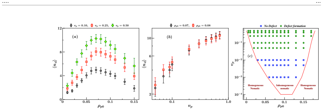
Numerical solution of the coupled hydrodynamic equations for the polar-apolar mixture reveals that, in an intermediate regime of polar activity and density, the system enters a dynamically disordered phase marked by high-density, chaotically evolving band-like structures together with continuous creation and annihilation of half-integer topological defects; this phase is spatiotemporally chaotic, as shown by the spectral properties of density fluctuations and a positive maximal Lyapunov exponent.
What carries the argument
The coupled hydrodynamic equations for the densities and order parameters of the polar and apolar components, solved numerically across parameter ranges to identify the intermediate chaotic regime.
If this is right
- The apolar species exhibits a non-monotonic response to polar density and activity.
- Spatiotemporal chaos appears through an inverse energy cascade typical of active systems rather than a direct cascade.
- Continual defect creation and annihilation occurs together with chaotic band evolution.
- The observed states broaden the set of possible complex transitions beyond those in living liquid crystal systems.
Where Pith is reading between the lines
- The chaotic regime could be used to control defect statistics by tuning only polar activity in an experimental mixture.
- Similar band-and-defect chaos may appear in other active mixtures such as colloidal rods combined with swimming bacteria.
- The Lyapunov exponent provides a practical diagnostic that could be tracked in future numerical studies of active mixtures to locate the onset of chaos.
Load-bearing premise
The chosen hydrodynamic equations fully capture the microscopic interactions and couplings between the polar and apolar components without requiring extra higher-order terms.
What would settle it
Direct measurement of the maximal Lyapunov exponent remaining zero (instead of positive) in either simulation or experiment at the reported intermediate polar densities and activities would falsify the spatiotemporal-chaos claim.
Figures


read the original abstract
Chaotic transitions in inertial fluids typically proceed through a direct energy cascade from large to small scales. In contrast, active systems, composed of self propelled units, inject energy at microscopic scales and therefore exhibit an inverse cascade, giving rise to distinctly unconventional flow patterns. Here, we investigate an active mixture consisting of both apolar and polar self driven components, a setting expected to display richer behaviours than those found in living liquid crystal (LLC) systems, where the apolar constituent is passive. Using numerical solutions of the corresponding hydrodynamic equations, we uncover a variety of complex dynamical states. Our results reveal a non-monotonic response of the apolar species to changes in the density and activity of the polar component. In an intermediate regime, reminiscent of LLC-induced disorder, the system develops a dynamically disordered phase characterised by high-density, chaotically evolving band-like structures and by the continual creation and annihilation of half integer topological defects. We show that this regime exhibits spatiotemporal chaos, which we quantify through two complementary measures: the spectral properties of density fluctuations and the maximal Lyapunov exponent. Together, these findings broaden the understanding of complex transitions in active matter and suggest potential experimental realisations in bacterial suspensions or synthetic microswimmer assemblies.
Editorial analysis
A structured set of objections, weighed in public.
Referee Report
Summary. The manuscript numerically solves hydrodynamic equations for a polar-apolar active mixture and reports a non-monotonic response of the apolar component to polar density and activity. In an intermediate regime the system enters a disordered phase with high-density chaotically evolving bands, continual creation/annihilation of half-integer defects, and spatiotemporal chaos diagnosed by density-fluctuation spectra and a positive maximal Lyapunov exponent.
Significance. If the numerical diagnostics prove robust under refinement, the work extends chaos studies in active matter beyond passive-apolar LLCs by demonstrating defect proliferation and inverse-cascade chaos in a fully active mixture, with potential experimental relevance to bacterial or microswimmer suspensions.
major comments (2)
- [Numerical results (Lyapunov exponent subsection)] Numerical results section on Lyapunov exponent: the reported positive maximal Lyapunov exponent is presented without grid-refinement studies, domain-size scaling, or checks against artificial viscosity and perturbation norm. In continuum active-matter PDEs the sign of this exponent is known to be sensitive to spatial discretization; absence of these controls leaves open the possibility that the observed chaos is a numerical artifact of under-resolved inverse cascades.
- [Results on density spectra] Section on spectral properties of density fluctuations: the power spectra are shown without ensemble averaging, error bars, or explicit convergence tests with respect to system size and integration time. This weakens the claim that the spectra independently confirm spatiotemporal chaos, especially given the non-monotonic parameter dependence highlighted in the abstract.
minor comments (2)
- [Abstract] Abstract: the statement that the disordered phase is 'reminiscent of LLC-induced disorder' would benefit from a one-sentence quantitative comparison to the relevant LLC literature (e.g., defect density or spectral exponent).
- [Figure captions] Figure captions: several panels lack explicit parameter values or grid resolution, making it difficult for readers to reproduce the reported states.
Simulated Author's Rebuttal
We thank the referee for their constructive and detailed report. We address each major comment below and will revise the manuscript to incorporate additional numerical controls that strengthen the evidence for spatiotemporal chaos.
read point-by-point responses
-
Referee: [Numerical results (Lyapunov exponent subsection)] Numerical results section on Lyapunov exponent: the reported positive maximal Lyapunov exponent is presented without grid-refinement studies, domain-size scaling, or checks against artificial viscosity and perturbation norm. In continuum active-matter PDEs the sign of this exponent is known to be sensitive to spatial discretization; absence of these controls leaves open the possibility that the observed chaos is a numerical artifact of under-resolved inverse cascades.
Authors: We agree that systematic convergence tests are necessary to exclude numerical artifacts in continuum models of active matter. In the revised manuscript we will add grid-refinement studies (halving the grid spacing), domain-size scaling (doubling the system size while keeping resolution fixed), and explicit checks varying artificial viscosity and perturbation norm. Additional simulations performed since submission confirm that the maximal Lyapunov exponent remains positive and quantitatively stable under these refinements, indicating that the reported chaos is not an artifact of under-resolution. revision: yes
-
Referee: [Results on density spectra] Section on spectral properties of density fluctuations: the power spectra are shown without ensemble averaging, error bars, or explicit convergence tests with respect to system size and integration time. This weakens the claim that the spectra independently confirm spatiotemporal chaos, especially given the non-monotonic parameter dependence highlighted in the abstract.
Authors: We acknowledge that ensemble averaging and convergence diagnostics would make the spectral evidence more robust. In the revised version we will include ensemble averages over at least five independent realizations, with error bars, together with explicit tests demonstrating convergence of the spectral shape with increasing system size and integration time. These additions will confirm that the inverse-cascade features and the non-monotonic dependence on polar density and activity are reproducible and not sensitive to finite-size or finite-time effects. revision: yes
Circularity Check
Numerical study applies independent diagnostics to simulated fields with no self-referential derivation
full rationale
The paper solves a set of hydrodynamic PDEs numerically for varying parameters and directly computes two independent diagnostics (Fourier spectra of density fluctuations and the maximal Lyapunov exponent) on the resulting spatiotemporal fields. No step fits a parameter to a data subset and then renames the output as a prediction, no self-citation supplies a load-bearing uniqueness theorem, and no ansatz or definition is smuggled in via prior work by the same authors. The central claim of an intermediate chaotic regime follows from the observed behavior of the simulated solutions rather than from any tautological reduction to the input equations or fitted quantities.
Axiom & Free-Parameter Ledger
free parameters (2)
- polar activity coefficient
- apolar density and activity parameters
axioms (1)
- domain assumption Hydrodynamic equations with polar-apolar couplings accurately describe the mixture at the chosen scales.
Lean theorems connected to this paper
-
IndisputableMonolith/Cost/FunctionalEquation.leanwashburn_uniqueness_aczel unclear?
unclearRelation between the paper passage and the cited Recognition theorem.
The evolution equations for the density and the symmetry-broken variable for both species are discussed below. ... ∂tρp = ∇·(Dρp ∇ρp − vp ρp P) ... ∂tQij = −ΓQ ∂FQ/∂Q + ... + γ(Pi Pj − ½ δij Pk Pk)
What do these tags mean?
- matches
- The paper's claim is directly supported by a theorem in the formal canon.
- supports
- The theorem supports part of the paper's argument, but the paper may add assumptions or extra steps.
- extends
- The paper goes beyond the formal theorem; the theorem is a base layer rather than the whole result.
- uses
- The paper appears to rely on the theorem as machinery.
- contradicts
- The paper's claim conflicts with a theorem or certificate in the canon.
- unclear
- Pith found a possible connection, but the passage is too broad, indirect, or ambiguous to say the theorem truly supports the claim.
Reference graph
Works this paper leans on
-
[1]
Vicsek T, Czir´ ok A, Ben-Jacob E, Cohen I and Shochet O 1995Physical Review Letters75 1226
-
[2]
Bechinger C, Di Leonardo R, L¨ owen H, Reichhardt C, Volpe G and Volpe G 2016Reviews of Modern Physics88045006
-
[3]
B¨ ar M, Großmann R, Heidenreich S and Peruani F 2020Annual Review of Condensed Matter Physics11441–466
-
[4]
thesis Indian Institute of Technology Hyderabad
Ganguly C 2013Aspects of Self-PropulsionPh.D. thesis Indian Institute of Technology Hyderabad
-
[5]
Vicsek T and Zafeiris A 2012Physics reports51771–140
-
[6]
Alberts B, Johnson A, Lewis J, Raff M, Roberts K and Walter P 2002 The self-assembly and dynamic structure of cytoskeletal filamentsMolecular Biology of the Cell. 4th edition(Garland Science)
work page 2002
-
[7]
Kolomeisky A B and Fisher M E 2007Annu. Rev. Phys. Chem.58675–695
-
[8]
Niu B, Wang Het al.2012Discrete Dynamics in Nature and Society2012
-
[9]
Shapiro J A 1995BioEssays17597–607
-
[10]
Jolles J W, Boogert N J, Sridhar V H, Couzin I D and Manica A 2017Current Biology27 2862–2868
-
[11]
Moreno Garc´ ıa C A, Maxwell T M, Hickford J and Gregorini P 2020Frontiers in Veterinary Science774
-
[12]
Gueron S, Levin S A and Rubenstein D I 1996Journal of Theoretical Biology18285–98
-
[13]
Wang X and Lu J 2019IEEE Circuits and Systems Magazine196–22
-
[14]
Sokolov A and Aranson I S 2012Physical review letters109248109 20
-
[15]
Dunkel J, Heidenreich S, Drescher K, Wensink H H, B¨ ar M and Goldstein R E 2013Physical review letters110228102
- [16]
-
[17]
Zhou S, Sokolov A, Lavrentovich O D and Aranson I S 2014Biophysical Journal106420a
-
[18]
Turiv T, Koizumi R, Thijssen K, Genkin M M, Yu H, Peng C, Wei Q H, Yeomans J M, Aranson I S, Doostmohammadi Aet al.2020Nature Physics16481–487
-
[19]
Kumar A, Galstian T, Pattanayek S K and Rainville S 2013Molecular Crystals and Liquid Crystals57433–39
-
[20]
Doostmohammadi A, Shendruk T N, Thijssen K and Yeomans J M 2017Nature communications815326
-
[21]
de la Cotte A, Pearce D J, Nambisan J, Puggioni L, Levy A, Giomi L and Fernandez-Nieves A 2025Proceedings of the National Academy of Sciences122e2512147122
-
[22]
Shankar S, Souslov A, Bowick M J, Marchetti M C and Vitelli V 2022Nature Reviews Physics 4380–398
-
[23]
Alert R, Casademunt J and Joanny J F 2022Annual Review of Condensed Matter Physics13 143–170
-
[24]
Genkin M M, Sokolov A, Lavrentovich O D and Aranson I S 2017Physical Review X7011029
-
[25]
Vats A, Yadav P K, Banerjee V and Puri S 2023Physical Review E108024701
-
[26]
Kemkemer R, Kling D, Kaufmann D and Gruler H 2000The European Physical Journal E1 215–225
-
[27]
Balasubramaniam L, M` ege R M and Ladoux B 2022Current Opinion in Genetics & Development73101897
-
[28]
Saw T B, Xi W, Ladoux B and Lim C T 2018Advanced materials301802579
-
[29]
Sampat P B and Mishra S 2021Physical Review E104024130
-
[30]
Mondal P S, Mishra P K, Vicsek T and Mishra S 2025Physica A: Statistical Mechanics and its Applications659130338 ISSN 0378-4371 URL https://www.sciencedirect.com/science/article/pii/S0378437124008483
-
[31]
Sharma A and Soni H 2025Soft Matter
-
[32]
De Gennes P G and Prost J 1993The physics of liquid crystals83 (Oxford university press)
-
[33]
Brochard F and De Gennes P 1970Journal de Physique31691–708
-
[34]
Lopatina L M and Selinger J V 2009Physical review letters102197802
-
[35]
Bisht K, Wang Y, Banerjee V and Majumdar A 2020Physical Review E101022706
-
[36]
Aditi Simha R and Ramaswamy S 2002Physical review letters89058101
-
[37]
Ramaswamy S, Simha R A and Toner J 2003Europhysics Letters62196
-
[38]
Bertin E, Chat´ e H, Ginelli F, Mishra S, Peshkov A and Ramaswamy S 2013New journal of physics15085032
-
[39]
Goldenfeld N 2018Lectures on phase transitions and the renormalization group(CRC Press)
-
[40]
Toner J 2022Active Matter and Non-Equilibrium Statistical Physics: Lecture Notes of the Les Houches Summer School, September 2018 112, eds. G52–101
work page 2018
-
[41]
Hohenberg P and Shraiman B I 1989Physica D: Nonlinear Phenomena37109–115 21
-
[42]
Wenzel D, Nestler M, Reuther S, Simon M and Voigt A 2021Computational Methods in Applied Mathematics21683–692
-
[43]
Delmarcelle T and Hesselink L 1994 The topology of symmetric, second-order tensor fields Proceedings Visualization’94(IEEE) pp 140–147
work page 1994
-
[44]
Cross M and Hohenberg P 1994Science2631569–1570
-
[45]
Packard N H, Crutchfield J P, Farmer J D and Shaw R S 1980Physical review letters45712
-
[46]
Lai Y C and Ye N 2003International Journal of Bifurcation and Chaos131383–1422
-
[47]
Skokos C H, Gottwald G A and Laskar J 2016Chaos detection and predictabilityvol 1 (Springer)
-
[48]
Berera A and Ho R D 2018Physical review letters120024101
-
[49]
Boffetta G and Musacchio S 2017Physical review letters119054102
-
[50]
Valsakumar M, Satyanarayana S and Sridhar V 1997Pramana4869–85
-
[51]
Marwan N and Braun T 2023Chaos: An Interdisciplinary Journal of Nonlinear Science33
-
[52]
Adenij A E 2024Communication in Physical Sciences11
-
[53]
Mishra S, Baskaran A and Marchetti M C 2010Physical Review E—Statistical, Nonlinear, and Soft Matter Physics81061916
-
[54]
Marchetti M C, Joanny J F, Ramaswamy S, Liverpool T B, Prost J, Rao M and Simha R A 2013Reviews of modern physics851143–1189
-
[55]
Mishra P K, Mondal P S, Jena P and Mishra S 2025New Journal of Physics27074602 URL https://doi.org/10.1088/1367-2630/adef71
-
[56]
Kantz H and Schreiber T 2003Nonlinear time series analysis(Cambridge university press)
-
[57]
Casdagli M 1992 Nonlinear forecasting, chaos and statisticsModeling Complex Phenomena: Proceedings of the Third Woodward Conference, San Jose State University, April 12–13, 1991 (Springer) pp 131–152
work page 1992
-
[58]
Fraser A M and Swinney H L 1986Physical review A331134
-
[59]
Kennel M B, Brown R and Abarbanel H D 1992Physical review A453403
-
[60]
Kaplan D T and Glass L 1992Physical review letters68427 22
discussion (0)
Sign in with ORCID, Apple, or X to comment. Anyone can read and Pith papers without signing in.