REVIEW 2 major objections 4 minor 47 references
Towards degeneracy breaking of early universe models
T0 review · 2 major / 4 minor · reviewed 2026-08-14 · deepseek-v4-flash
Pith's one-line read Measuring the time variation of particle and Planck masses could break the degeneracy among conformally related early-universe models, identifying which scenario is physically realized.
desk verdict The parametrization idea is genuinely worth exploring, but the central integral relation behind the parameter-space plots is inconsistent with the paper's own definitions, so the I-group figures do not show what the paper claims. read the letter →
The pith
A machine-rendered reading of the paper's core claim, the machinery that carries it, and where it could break.
The reading
What carries the argument
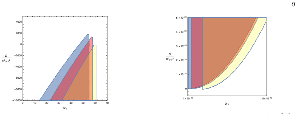
The machinery is the set of frame-invariant variables introduced by Ijjas and Steinhardt: α_m = a m/$M_Pl^{0}$, α_Pl = a M_Pl/$M_Pl^{0}$, Θ_m = (H + ṁ/m)/M_Pl, Θ_Pl = (H + Ṁ_Pl/M_Pl)/M_Pl, together with the associated slow-roll parameters ε_m and ε_Pl. These variables are equal in all conformal frames, yet their signs and magnitudes differ by scenario, as summarized in Table I. The paper's specific tool is the integral relation (80) between ε_m and ε_Pl, which after differentiation becomes Eq. (81) and, under the parametrization (83) for the Einstein-frame background, yields the closed expressions (84) that map scenarios to regions of the parameter space spanned by D/γ and Ḋ/($M_Pl^{0}$ γ²).
What would settle it
Take a concrete nonminimal coupling function, e.g., f(t)=α $t^{{2β}}$, evolve the exact background equations in both Jordan and Einstein frames, compute ε_m and ε_Pl directly from their definitions (77), and test whether the integral relation (80) holds; if it fails for even one such model, the derived region boundaries do not follow from the stated premises. Independently, a future measurement of Ṁ_Pl/M_Pl and ṁ/m at early times that falls in no predicted region for any N_E and ε_E would falsify the classification's completeness.
Extended reading notes
Core claim
The central claim is that a measurement of the two frame-invariant combinations D/γ and Ḋ/($M_Pl^{0}$ γ²), together with the Einstein-frame e-folding number N_E and slow-roll parameter ε_E, is sufficient to decide which early-universe scenario actually occurred, even when the primordial spectra are conformally degenerate. The paper derives parametrized expressions for the Jordan-frame Hubble-like variable Θ_m and slow-roll parameter ε_m in terms of these parameters, and plots the regions corresponding to slow contraction and slow expansion for both the I-group (dual to inflation) and the M-group (dual to matter contraction). It finds that the I-group generically requires a large running of the Planck mass, whereas the M-group allows small running but is exponentially sensitive to N_E. For the trivial case D=0, general relativity is recovered and the Jordan frame coincides with the Einstein frame.
Load-bearing premise
The entire parameter-space classification rests on an integral relation between the frame-invariant slow-roll parameters, Eq. (80), which the paper states without proof and then differentiates to obtain the expressions used to draw the region plots.
Editorial extensions
If this is right
- If the regions are correct, future constraints on the early-time running of the Planck mass and particle mass—for instance from standard-clock observations—would uniquely select the physical conformal frame and thereby the actual early-universe scenario.
- Within the I-group, the non-detection of a large Planck-mass running (D close to 0) would leave inflation as the only possibility in the Jordan frame, recovering the ordinary GR description.
- Within the M-group, the allowed regions shift by orders of magnitude when N_E changes by one e-fold, so a precise determination of the e-folding number is required before the scenario can be identified from these parameters.
- The concrete coupling-function analysis shows that for exponential f(t), the Jordan frame always behaves like inflation (ε_m=0, Θ_m>0) for both groups, so such models cannot be distinguished by this method alone; power-law and polynomial f(t) do yield distinguishing slow-roll/slow-expansion regions.
- The parametrized approach can be applied to any nonminimal coupling function, so future models can be classified by computing their effective f(t) and locating them in the same parameter space.
Reading between the lines
- Editorial inference: the unproved integral relation (80) is the linchpin of the region maps; a direct derivation from the definitions (77) or a numerical check for individual models would settle whether the boundaries are trustworthy.
- Editorial inference: because the frame-invariant variables track the ratio m/M_Pl, the same classification could in principle be applied to late-time scalar-tensor theories, where local tests of equivalence-principle violation already set tight bounds on ṁ/m and Ġ/G; those bounds could be projected onto the same parameter space to exclude early-universe scenarios that require large running.
- Editorial inference: the method assumes a single canonical scalar field with c_s²=1; extending the region analysis to multi-field or non-canonical sound-speed models would test whether the scenario separation survives in more general settings.
- Editorial inference: the claimed exponential sensitivity of the M-group regions to N_E suggests that observations constraining the duration of the nonstandard phase (e.g., BBN bounds on e-folds) will matter as much as direct measurements of mass running for the degeneracy-breaking program.
Editorial analysis
A structured set of objections, weighed in public.
Referee Report
Summary. The paper addresses the conformal-frame degeneracy among early-universe scenarios (slow-roll inflation, matter contraction, slow contraction, and slow expansion) that can produce nearly scale-invariant primordial spectra. Using the frame-invariant variables of Ijjas and Steinhardt, the authors parametrize the difference between Jordan- and Einstein-frame descriptions in terms of the time variation of the particle mass and the Planck mass. They then divide the parameter space of the dimensionless combinations D/γ and Ḋ/(M_Pl^0 γ^2) into regions corresponding to the different scenarios, presenting these regions in Figs. 1–6, and they analyze three concrete coupling functions f(t). The central claim is that future measurements of these mass-variation parameters could identify which conformal frame is physical and thereby break the degeneracy between the scenarios.
Significance. If the parameter-space predictions were correct, the paper would provide a concrete, falsifiable route toward distinguishing conformally dual early-universe models, a question of current interest. The review of the perturbation spectra in Section II is standard and serves as a useful synthesis. The concrete coupling-function examples in Section IIIC are internally consistent and appear to be independent of the main parametrization. However, the central derivation connecting the frame-invariant slow-roll parameters ε_m and ε_Pl is flawed, and the resulting parameter-space regions, which constitute the main quantitative result, are not trustworthy. The paper is therefore not acceptable in its present form.
major comments (2)
- [Sec. IIIA, Eqs. (77)–(84)] The relation (80) is stated without derivation and is inconsistent with the defining equations (77)–(79). As written, Eq. (80) is dimensionally unbalanced, and differentiating it does not reproduce Eq. (81). More importantly, Eq. (81) disagrees with the direct definition of ε_m when the paper's own initial condition M_Pl^0 t_E^0 = 1 is used. For example, take M_Pl^0 = 1, γ = 1, constant ε_E = ε_Pl = ε = 0.01, and D = Δ_M − Δ_m = −Δ_m so that d ln m/dt = −D and Ḋ = 0. Then from Eq. (79), Θ_m = 1/(ε t) − D. Evaluating Eq. (77) directly gives ε_m = (ε − D ε t + D^2 ε^2 t^2)/(1 − D ε t)^2. With N_E = 60, the e-folding relation gives t_E = t_E^0 e^{ε N_E} = e^{0.6} = 1.822. Direct evaluation with t = 1.822 and D = 50 gives ε_m ≈ −9. In contrast, Eq. (84) uses the integral ∫ ε_Pl M_Pl^0 dt_E = ε(e^{ε N_E} − 1) = 0.01(e^{0.6} − 1) = 0.00822 and gives ε_m ≈ −0.7. Thus the two expressions differ by more than an order of magnitude and can place the same parameter point in different scenario regions of Figs. 1–6. Since the division of parameter space in Section IIIB rests on Eq. (84), the central claim of the paper is unsupported.
- [Sec. IIIA, Eq. (80)] The paper never proves Eq. (80); the text says only that 'one can obtain' it. Appendix A derives the frame-invariant variables but does not derive this integral relation. Given that the relation is load-bearing for the main result, a complete derivation is required, and the derivation must be consistent with the initial condition M_Pl^0 t_E^0 = 1 used in Eq. (84). The current text leaves the reader unable to verify the central step.
minor comments (4)
- [Eq. (80)] The equation is dimensionally inconsistent as printed: the denominator subtracts a term of dimension [M^2 T] from a term of dimension [M]. This should be corrected and the notation clarified.
- [Eq. (84)] The placement of parentheses in the last term of Eq. (84) is ambiguous; it should read (Ḋ/M_Pl^0 − Δ_m D)/γ^2 multiplied by ε_E (e^{ε_E N_E} − 1)^2, with all factors explicitly shown.
- [Table I] The caption contains the typo 'expanstion' instead of 'expansion'.
- [Eq. (35)] The inequality 0 < 3 + 2k(φ) f(φ)/f_{,φ}^2 < ε_E < 1 is hard to parse; a brief derivation or a reference to the condition in [1] would improve readability.
Circularity Check
No circularity; the central parameter-space maps are derived from independently motivated scenario conditions, and the only self-citation is a non-load-bearing consistency check.
full rationale
The paper's claimed result—that future constraints on D/γ and Ḋ/(M_Pl^0 γ²) would localize a scenario—is conditional and is not obtained by fitting a parameter and then 'predicting' a closely related quantity. The regions in Sec. IIIB are computed by inserting the independently established scenario conditions of Table I (e.g., ε_m ≃ 0 for inflation-dual, ε_m ≥ 3 for slow contraction, ε_m ≪ −1 for slow expansion) into the parametrized expressions of Eq. (84). The frame-invariant variables themselves are not assumed as black boxes: they are re-derived in Appendix A from the conformal transformation, and the only self-citation [10] appears as a check that 'the above results are consistent with our previous works,' which is not load-bearing. The main caveat is that Eq. (80), the integral relation connecting ε_m and ε_Pl, is stated with 'one can obtain' and no derivation; the skeptic's example suggests it may be inconsistent with the direct definitions (77)–(79) for the lower limit chosen in Sec. IIIA. However, an unproved or incorrect intermediate step is a correctness risk, not a circularity: the conclusion is not identical to an input by construction, no fitted datum is relabeled as a prediction, and no load-bearing argument reduces to a self-citation. Hence the circularity score is 0.
Assumptions & free parameters
free parameters (4)
- ε_E (Einstein-frame slow-roll parameter) =
chosen as 0.010, 0.0111, 0.0125 for I-group and 1.5 for M-group in the plots
- N_E (Einstein-frame e-folding number) =
chosen as 60, 55, 50 for I-group and 19, 20, 21 for M-group
- D/γ and Ḋ/(M_Pl^0 γ^2)
- β (power-law exponent in f = α t^{2β}) and ρ (combination of α, β in polynomial f = (α+βt)^2)
assumptions (4)
- domain assumption Conformal transformations leave superhorizon curvature perturbations and power spectra unchanged, so conformally related models are observationally degenerate.
- domain assumption The Einstein-frame background is exactly power-law, a_E ∝ t_E^{1/ε_E}, with constant ε_E over the observable e-folding range.
- domain assumption The no-ghost and stability conditions of Eq. (35) from Ijjas and Steinhardt (2015) are adopted.
- standard math The perturbation spectra for inflation, matter contraction, slow contraction, and slow expansion are taken from the cited literature and are not re-derived.
Cite this review
Pith. "Pith review of Towards degeneracy breaking of early universe models." pith.science (2026). https://pith.science/paper/BRRSCXEZ
@misc{pith2026190803695,
  author       = {Pith},
  title        = {Pith review of: Towards degeneracy breaking of early universe models},
  year         = {2026},
  howpublished = {\url{https://pith.science/paper/BRRSCXEZ}},
  note         = {Machine review of arXiv:1908.03695}
}
read the original abstract
There are many possibilities of scenarios in the early universe, which can give rise to the same observational signals due to the degeneracy among each other, caused by equivalence under the conformal transformations. In order to break the degeneracy, in this paper we take into account the so-called "frame-invariant variables" proposed by A. Ijjas and P. J. Steinhardt in \cite{Ijjas:2015zma}. We discuss how the different scenarios will distribute in different parametric space constructed from those variables, waiting for the judgement of real observations in the future. Several concrete models with explicit non-minimal coupling functions are also discussed.
Figures


Figures from the paper (1 more)

Reference graph
Works this paper leans on
-
[1]
× 10-15 1.5 × 10⁻¹² 0
-
[2]
Similar to the scalar case, the initial condition of v can be obtained from Eq
Moreover, a∼ τ 1/(ϵinf−1) leads to a′′ a → 2−ϵinf (ϵinf−1)2τ 2 , which gives the solution: v =dinf 1 √ |τ|Hν(|kτ|) , dinf 2 √ |τ|H−ν(|kτ|) , (16) and also γ = √ 2v a =dinf 1 2√πHkν|τ| 3 2 +ν , dinf 2 2√πHk−ν|τ| 3 2−ν (17) in superhorizon region. Similar to the scalar case, the initial condition of v can be obtained from Eq. (15) by considering the large k...
-
[3]
Since for ϵmc ≃ 3/2, ν ≃ 3/2, and from Eq. (24) one can see that first mode is con- stant while the second mode is growing [39]. So the spec- trum and spectral index will be determined by the second mode: PS mc ≡ k3 2π2|ζ|2 = H 2 8π2ϵmc |kτ|3−2ν , (25) nS mc ≡ 1 +d lnPS mc d lnk = 5− 2 ϵmc− 1 , (26) which is nearly scale-invariant as ϵmc is close to 3/2. M...
-
[4]
J. L. Lehners, Phys. Rept. 465, 223 (2008) [arXiv:0806.1245 [astro-ph]]
arXiv 2008
-
[5]
× 10-24 D/γ D M0pl γ2 FIG. 5: The region in parameter space of {D/γ, ˙D/(M 0 plγ2)} which corresponds to slow-contraction in Jordan frame while matter-contraction in Einstein frame (M-group). The blue, red, yellow regions corresponds to NE = 21, 20, 19 respec- tively, withεE = 3/2. -2.2 × 10⁻¹² 1. × 10-12 -5. × 10-24 -4. × 10-24 -3. × 10-24 -2. × 10-24 -...
-
[6]
Therefore, Θ m > 0 for β >−1 or β <−1/(1−ϵE) while Θm < 0 for only narrow range of −1/(1−ϵE) < β <−1. Moreover, for large value of β, we have ϵ≈ ϵE, which gives rise to inflation-like behavior in Jordan frame. The phase space for slow-contraction and slow expansion will be constrained to the regions of (−1/(1− ϵE),−(1−ϵE/3)/(1−ϵE)] and [−(1+ϵE)/(1−ϵE),−1/(...
-
[7]
Therefore, Θ m > 0 for ρ< −tE or ρ> (εE− 2)tE/2, while Θm < 0 for ( εE− 2)tE/2 < ρ <−tE. More- over, whenρ =εEtE(εE + 1)/[2(2εE− 1)]−tE, we have εm ≈ εE, which gives rise to inflation-like behavior in Jordan frame. Note that although we can make Θm > 0, there is no way to get slow-contraction phase, since the condition ofϵm > 3 cannot be satisfied. The phas...
-
[8]
A. Ijjas and P. J. Steinhardt, JCAP 1510, no. 10, 001 (2015) doi:10.1088/1475-7516/2015/10/001 [arXiv:1507.03875 [astro-ph.CO]]
work page Pith review arXiv 2015
Show all 47 references
-
[9]
R. A. Alpher, H. Bethe and G. Gamow, Phys. Rev. 73, 803 (1948); G. Gamow, Phys. Rev. 70, 572 (1946)
1948
-
[10]
Novello and S
M. Novello and S. E. P. Bergliaffa, Phys. Rept. 463, 127 (2008) [arXiv:0802.1634 [astro-ph]]
2008 arXiv
-
[11]
A. H. Guth, Phys. Rev. D 23, 347 (1981)
1981
- [12]
-
[13]
P. A. R. Ade et al. [Planck Collaboration], Astron. Astro- phys. 594, A17 (2016) [arXiv:1502.01592 [astro-ph.CO]]
2016 arXiv
-
[14]
Finelli and R
F. Finelli and R. Brandenberger, Phys. Rev. D 65, 103522 (2002) [hep-th/0112249]
2002 arXiv
-
[15]
Wands, Phys
D. Wands, Phys. Rev. D 60, 023507 (1999) [gr- qc/9809062]
1999
-
[16]
Y. S. Piao, arXiv:1109.4266 [hep-th]; Y. S. Piao, arXiv:1112.3737 [hep-th]; Y. Cai and Y. S. Piao, JHEP 1603, 134 (2016) [arXiv:1601.07031 [hep-th]]
2016 arXiv
-
[17]
Qiu, JCAP 1206, 041 (2012) [arXiv:1204.0189 [hep-ph]]; T
T. Qiu, JCAP 1206, 041 (2012) [arXiv:1204.0189 [hep-ph]]; T. Qiu, Phys. Lett. B 718, 475 (2012) [arXiv:1208.4759 [astro-ph.CO]]
2012 arXiv
-
[18]
Finelli, Phys
F. Finelli, Phys. Lett. B 545, 1 (2002) [hep-th/0206112]; A. Notari and A. Riotto, Nucl. Phys. B 644, 371 (2002) [hep-th/0205019]
2002 arXiv
-
[19]
A. D. Linde, Phys. Lett. B 108, 389 (1982)
1982
-
[20]
A. A. Starobinsky, Phys. Lett. B 91, 99 (1980)
1980
-
[21]
Quintin, Z
J. Quintin, Z. Sherkatghanad, Y. F. Cai and R. H. Bran- denberger, Phys. Rev. D 92, no. 6, 063532 (2015) [arXiv:1508.04141 [hep-th]]
2015 arXiv
-
[22]
K. E. Kunze and R. Durrer, Class. Quant. Grav.17, 2597 (2000) [arXiv:gr-qc/9912081]; J. K. Erickson, D. H. Wes- ley, P. J. Steinhardt and N. Turok, Phys. Rev. D 69, 063514 (2004) [arXiv:hep-th/0312009]; B. Xue and P. J. Steinhardt, Phys. Rev. Lett. 105, 261301 (2010) [arXiv:10...
2000 arXiv
-
[23]
Khoury, B
J. Khoury, B. A. Ovrut, P. J. Steinhardt and N. Turok, Phys. Rev. D 64, 123522 (2001) [arXiv:hep-th/0103239]; J. Khoury, B. A. Ovrut, N. Seiberg, P. J. Steinhardt and N. Turok, Phys. Rev. D 65, 086007 (2002) [arXiv:hep- th/0108187]; J. Khoury, B. A. Ovrut, P. J. Stein- hardt a...
2001 arXiv
-
[24]
Khoury and P
J. Khoury and P. J. Steinhardt, Phys. Rev. Lett. 104, 091301 (2010) [arXiv:0910.2230 [hep-th]]
2010 arXiv
-
[25]
Elizalde, J
E. Elizalde, J. Haro and S. D. Odintsov, Phys. Rev. D 91, no. 6, 063522 (2015) [arXiv:1411.3475 [gr-qc]]
2015 arXiv
-
[26]
Hinterbichler and J
K. Hinterbichler and J. Khoury, JCAP 1204, 023 (2012) [arXiv:1106.1428 [hep-th]]; M. Libanov, S. Mironov and V. Rubakov, Phys. Rev. D 84, 083502 (2011) [arXiv:1105.6230 [astro-ph.CO]]; P. Creminelli, Phys. Rev. D 85, 041302 (2012) [arXiv:1108.0874 [hep-th]]
2012 arXiv
-
[27]
Wetterich, Phys
C. Wetterich, Phys. Dark Univ. 2, 184 (2013) [arXiv:1303.6878 [astro-ph.CO]]; C. Wetterich, Phys. Rev. D 89, no. 2, 024005 (2014) [arXiv:1308.1019 [astro- ph.CO]]; C. Wetterich, Phys. Lett. B 736, 506 (2014) [arXiv:1401.5313 [astro-ph.CO]]
2013 arXiv
-
[28]
Y. S. Piao and E. Zhou, Phys. Rev. D 68, 083515 (2003) [hep-th/0308080]
2003 arXiv
-
[29]
R. H. Brandenberger, Class. Quant. Grav. 28, 204005 (2011) [arXiv:1105.3247 [hep-th]]
2011 arXiv
-
[30]
Y. S. Piao, Phys. Lett. B 701, 526 (2011) [arXiv:1012.2734 [hep-th]]
2011 arXiv
-
[31]
A. R. Liddle and S. M. Leach, Phys. Rev. D 68, 103503 (2003) [astro-ph/0305263]
2003 arXiv
-
[32]
Avilez and C
A. Avilez and C. Skordis, Phys. Rev. Lett. 113, no. 1, 011101 (2014) doi:10.1103/PhysRevLett.113.011101 [arXiv:1303.4330 [astro-ph.CO]]
2014 arXiv
-
[33]
J. D. Barrow and J. Magueijo, Phys. Rev. D 72, 043521 (2005) [astro-ph/0503222]
2005 arXiv
-
[34]
D. F. Mota and D. J. Shaw, Phys. Rev. D 75, 063501 (2007) [hep-ph/0608078]
2007 arXiv
-
[35]
C. G. Scoccola, M. E. Mosquera, S. J. Landau and H. Vucetich, Astrophys. J. 681, 737 (2008) [arXiv:0803.0247 [astro-ph]]
2008 arXiv
-
[36]
S. J. Landau, M. E. Mosquera, C. G. Scoccola and H. Vucetich, Phys. Rev. D 78, 083527 (2008) [arXiv:0809.2033 [astro-ph]]
2008 arXiv
-
[37]
C. G. Scccola, S. J. Landau and H. Vucetich, Mem. Soc. Ast. It. 80, no. 4, 814 (2009) [Highlights Astron. 15, 307 (2010)] [arXiv:0910.1083 [astro-ph.CO]]
2009 arXiv
-
[38]
Zahn and M
O. Zahn and M. Zaldarriaga, Phys. Rev. D 67, 063002 (2003) doi:10.1103/PhysRevD.67.063002 [astro- ph/0212360]
2003
-
[39]
Note that here H scales as τ−3
-
[40]
J. X. Li, F. Q. Wu, Y. C. Li, Y. Gong and X. L. Chen, Res. Astron. Astrophys. 15, no. 12, 2151 (2015) doi:10.1088/1674-4527/15/12/003 [arXiv:1511.05280 [astro-ph.CO]]
2015 arXiv
-
[41]
J. Ooba, K. Ichiki, T. Chiba and N. Sugiyama, Phys. Rev. D 93, no. 12, 122002 (2016) doi:10.1103/PhysRevD.93.122002 [arXiv:1602.00809 [astro-ph.CO]]
2016 arXiv
-
[42]
Alonso, E
D. Alonso, E. Bellini, P. G. Ferreira and M. Zu- malacrregui, Phys. Rev. D 95, no. 6, 063502 (2017) doi:10.1103/PhysRevD.95.063502 [arXiv:1610.09290 [astro-ph.CO]]
2017 arXiv
-
[43]
Chen and M
X. Chen and M. H. Namjoo, Phys. Lett. B 739, 285 (2014) [arXiv:1404.1536 [astro-ph.CO]]; X. Chen, M. H. Namjoo and Y. Wang, JCAP 1502, no. 02, 027 (2015) [arXiv:1411.2349 [astro-ph.CO]]. 13
2014 arXiv
-
[44]
X. Chen, M. H. Namjoo and Y. Wang, JCAP 1602, no. 02, 013 (2016) [arXiv:1509.03930 [astro-ph.CO]]
2016 arXiv
-
[45]
The constant is exact, sinceH also has a dependence ofτ, i.e.H∼τ−ϵinf/(ϵinf−1), which conpensate the deviation of ν from−3/2
-
[47]
adiabatic mech- anism
There are however some mechanism call “adiabatic mech- anism” to obtain scale-invariant perturbations by evolv- ing the slow-varying parameter ε, see [23]. However, we will not discuss this situation in the current status
-
[60]
For example, Ref
However, for M-group, since the Big-Bang prob- lems are considered in other mechanisms, the constraint on NE mainly comes from observation, therefore can be much shorter than 60. For example, Ref. [24] gives a minimum e-folding number of 18 by BBN constraint on non-standard co...
2000
Reviewed August 14, 2026 · model on record in the stance chip above.
Discussion (0). Continue with ORCID to comment.