REVIEW 4 major objections 5 minor 26 references
An Active Learning-Based Streaming Pipeline for Reduced Data Training of Structure Finding Models in Neutron Diffractometry
T0 review · 4 major / 5 minor · reviewed 2026-08-07 · deepseek-v4-flash
Pith's one-line read An active learning policy trains neutron structure-finding models with about 75% less data.
desk verdict Plausible data-reduction result, but the missing random-sampling phased control means the AL policy is not isolated as the cause; the systems work is the strongest part. read the letter →
The pith
A machine-rendered reading of the paper's core claim, the machinery that carries it, and where it could break.
The reading
What carries the argument
The load-bearing object is the sampling distribution over unit-cell parameter space, defined as a prior-weighted Gaussian mixture placed on an interpolated surface of the model's estimated heteroscedastic uncertainty: $p(y) \propto p_Y(y) \sum_n \hat{\sigma}^2(S(\bar y_n);D) \, e^{-(y-\bar y_n)^2/2\tau^2}$ over a study set of roughly equally spaced parameters. This distribution redirects simulation effort toward Bragg profiles the current model predicts least well, while the prior $p_Y$ suppresses outliers that are uncertain but unrepresentative. The streaming workflow is a secondary mechanism: it overlaps training tasks on GPUs with simulation tasks on CPUs and uses NUMA-aware CPU/GPU binding to recover otherwise idle resources.
What would settle it
Run the serial AL workflow and a uniform-random-sampling workflow with the same total number of simulated samples, the same phase schedule, and the same epoch counts; if the random sampler reaches equal accuracy at equal data volume, the AL policy's data-reduction claim is not supported. A second check is to compare predicted $\hat\sigma^2(S(y);D)$ against the empirical squared error $\|y-\hat y(S(y);D)\|^2$ on a dense held-out grid: large deviations in sparse regions would indicate the sampling distribution is built on miscalibrated uncertainties.
Extended reading notes
Core claim
On the authors' own terms, the central discovery is that querying new simulation points from a distribution proportional to the model's estimated heteroscedastic uncertainty, rather than from a uniform grid, collapses the data requirement for training a multitask classifier-regressor of crystal structure. After four active learning phases, the same model reaches baseline accuracy with about 27,000 to 54,000 training samples where the uniform baseline needs roughly four to six times more, and it does so with lower classification loss and mean squared error. The paper also demonstrates that a streaming workflow, which splits each simulation batch between a serial analysis pipeline and a concurrent simulation task, matches the serial AL workflow's accuracy while cutting wall-clock training time by about 13% to 24% across two platforms and dataset scales.
Load-bearing premise
The whole data-reduction result rests on the model's estimated uncertainty $\hat\sigma^2$ being a trustworthy proxy for true prediction error in regions the model has seen little data: if the uncertainty estimate is miscalibrated or biased low in sparse regions, the sampler will not consistently choose the most informative next simulations.
Editorial extensions
If this is right
- Structure-finding models for neutron diffraction can be trained with roughly a quarter of the simulated data, shortening the data-generation phase from days to hours for a given accuracy target.
- The same model checkpoint reaches lower classification loss and MSE than uniform-grid training at equal or larger dataset sizes, so practitioners can either cut simulation cost or improve model quality at a fixed budget.
- A pseudo-streaming workflow that overlaps simulation with training recovers about 13% to 24% of wall-clock time on CPU+GPU systems without changing the final model accuracy.
- The authors state that the pipeline carries over directly to X-ray diffractometry and is being applied to other simulation-steered ML workloads such as diffusion-equation surrogates and detector design.
Reading between the lines
- A natural next test, not performed in the paper, is to compare the AL policy against random sampling with identical total data and epoch budgets; such a comparison would isolate how much of the gain comes from query selection rather than from simply training on more data.
- The policy's effectiveness presumably depends on the uncertainty estimator being calibrated in sparse regions; a calibration check comparing predicted $\hat\sigma^2$ with empirical squared error on held-out parameter regions would tell whether the gains persist outside the tested symmetry classes.
- One could extend the study-set interpolation to adaptive spacing, shrinking $\tau$ or locally refining the study set in high-uncertainty regions, which might further reduce the number of simulated profiles needed.
- The streaming design suggests that other three-phase loops of simulate, train, and select could reuse the same overlap pattern whenever simulation and training have different hardware affinities.
Editorial analysis
A structured set of objections, weighed in public.
Referee Report
Summary. This manuscript proposes a batch-mode active learning (AL) policy based on heteroscedastic uncertainty estimates for training structure-prediction models from simulated neutron diffraction patterns. The policy defines a proposal distribution over lattice parameters proportional to model uncertainty (Eq. 4), and the authors integrate it into a serial phase-based workflow and a pseudo-streaming workflow that overlaps GSAS-II simulation with GPU training. Experiments on three crystallographic symmetry classes compare a four-phase AL serial workflow against a uniform-sampling baseline (Section V-E) and compare serial vs streaming workflows on Polaris and Perlmutter (Section V-F). The central claims are that the AL workflow trains the same model with about 75% less data while improving accuracy, and that the streaming workflow reduces end-to-end training time by about 12-24% with no accuracy loss.
Significance. If the data-reduction claim is valid, the paper is a useful practical contribution: it combines uncertainty-based AL with a streaming HPC workflow for an important scientific inverse problem, and it reports experiments on real GSAS-II simulations with six seeds in E1, open-source code, and two leadership-class platforms. The 4-6x data reduction relative to uniform sampling would be significant for practitioners. However, the current evidence does not isolate the AL selection mechanism from the warm-started, multi-phase training protocol, and the theoretical justification in Section II is only asserted. These issues must be resolved before the central claims can be accepted as stated.
major comments (4)
- [Section V-E; Section IV-A/IV-B; Table II] The comparison that supports the 75% data-reduction claim is confounded. The baseline workflow is a one-shot bulk uniform sampler, while the AL serial workflow is trained in four phases with warm-started weights and a decreasing epoch budget (Table II: 400/300/250/200 epochs per phase) and validation-based model selection. The observed advantage of the AL workflow after phase 1 (27k samples) and phase 3 (54k samples) over the baseline could therefore be produced by the phased warm-starting, the larger cumulative number of training epochs, or the model-selection rule, rather than by the uncertainty-proportional distribution in Eq. (4). Please add a control arm that uses the same phase structure, batch sizes, epoch schedule, warm-starting, and validation selection as the AL workflow but draws each phase's samples uniformly (or by random sampling from the same study set). Without such a control, the data-reduction claim is not established.
- [Section II, Eq. (4)] The paper states, 'We then show that a model trained on this new set will have lower total uncertainty,' but no theorem, proof, or citation is provided. This is the core mechanism of the AL policy: sampling from p in Eq. (4) is claimed to reduce sigma^2(D) in Eq. (2). Please provide a precise statement with conditions under which this monotone improvement holds, or reframe Eq. (4) as an unproven heuristic and validate it empirically (e.g., show that selected batches reduce held-out error faster than uniform batches in matched-protocol experiments). The current text overclaims logical support for the policy.
- [Section II, III; Eq. (6)] The heteroscedastic uncertainty estimate sigma-hat^2, which drives Eq. (4), is never calibrated or validated as a proxy for the true prediction error sigma^2 in Eq. (1). The manuscript states a regularity requirement ('strictly positive and bounded') but provides no experiment showing that sigma-hat^2 is informative about actual squared error, particularly in sparse regions of parameter space where AL sampling is most active. The accuracy comparisons in Section V report only classification loss and MSE (Eqs. 6-7), not uncertainty calibration. Please add a calibration analysis - for example, bin held-out predictions by sigma-hat^2 and compare mean sigma-hat^2 with mean squared error, and show that the AL selection actively shifts training mass toward high-error regions.
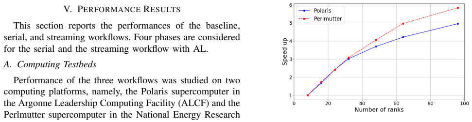
- [Section V-F2, Tables IV and V] The E2 scalability results, which are used to support the streaming workflow's 12-24% speedup, are based on a single run per configuration. Without multiple seeds or repeated runs, the reported differences (e.g., 1.24 vs 1.19 speedup across node counts) cannot be distinguished from noise. At minimum, report variance or confidence intervals for E2 or clearly mark these as pilot results. This does not invalidate the E1 finding, but it limits the strength of the generalizability claim in the conclusions.
minor comments (5)
- [Eq. (6)] Equation (6) has unbalanced parentheses and uses y(x_n) where the model output appears intended as y-hat(x_n); please correct the notation.
- [Table II] The formatting of the E2 parameter ranges is ambiguous: 'a for cubic [3.5, 4.5) [2.5, 5.5)' and 'a and c for trigonal/tetragonal [3.8, 4.2) [3.5, 4.5)' appear as two bracketed intervals with no clear column separation; please restate the ranges in separate rows or columns with explicit parameter names.
- [Section VI] The conclusion misspells 'diffractrometry' (should be 'diffractometry'), and the abstract contains a subject-verb agreement issue ('The potential ... have been reported'); a light proofread is recommended.
- [Section V-B; Table II] The text says the number of epochs in each phase is approximately inversely proportional to sqrt(N_tot), but Table II lists constant epoch counts (400/300/250/200) rather than values computed from that formula; please clarify how the schedule is derived.
- [Acknowledgments] The acknowledgments mention an earlier IEEE BigData 2024 paper and a ROSE port; the manuscript should explicitly disclose this relationship and state what new material is presented in this version.
Circularity Check
No circular derivation; the 75% data-reduction claim is an externally benchmarked empirical result, though self-cited uncertainty estimation and a missing random-control condition create a modest attribution burden.
full rationale
The paper's central data-reduction claim is an empirical benchmark, not a mathematical entailment: the AL workflow's accuracy is measured on a fixed held-out test set generated by GSAS-II, while the AL sampling distribution in Eq. (4) is used only to select the next training batch and does not enter the test-set construction. The comparison to a uniform-sampling baseline in Section V-E is therefore a genuine experiment rather than an identity, and no equation in Sections II-V reduces the 4-6x data advantage to the definition of p(y) by construction. The self-cited base model [1] and heteroscedastic uncertainty estimator [20] are used as pre-existing building blocks; although [20] provides the sigma-hat^2 proxy whose strict positivity and boundedness are only asserted in Section II, and not validated, that is an unsupported assumption and an attribution gap, not a circular reduction. The main caveat is that Section V-E compares the phased, warm-started, decreasing-epoch AL protocol against a one-shot bulk baseline, so the observed data saving is not isolated to the uncertainty-weighted selection rule; a random-sampling control with the same phased schedule is absent. This affects causal attribution and correctness risk, but it does not make the '75% less data' result equivalent to the AL policy by definition. Overall, no circular step is exhibited, so the circularity score is low.
Assumptions & free parameters
free parameters (3)
- tau (Gaussian spread in Eq. 4) =
not reported
- Epoch schedule per phase =
400, 300, 250, 200
- Streaming phase split ratio 0.6 =
0.6
assumptions (4)
- domain assumption The heteroscedastic uncertainty estimate sigma-hat^2 from [20] faithfully approximates the true conditional error sigma^2 and is strictly positive and bounded on Y.
- domain assumption GSAS-II simulated Bragg profiles are a valid proxy for the inverse mapping S^{-1}, so that performance on simulated test data reflects performance on the learning task.
- domain assumption The user-supplied prior pY over unit-cell parameters is representative of the natural population and does not bias sampling away from informative regions.
- ad hoc to paper The study set S is sufficiently dense and equally spaced for Eq. (4) to reconstruct the uncertainty surface without artificial mass accumulation.
Cite this review
Pith. "Pith review of An Active Learning-Based Streaming Pipeline for Reduced Data Training of Structure Finding Models in Neutron Diffractometry." pith.science (2026). https://pith.science/paper/DEL4W2PA
@misc{pith2026250611100,
  author       = {Pith},
  title        = {Pith review of: An Active Learning-Based Streaming Pipeline for Reduced Data Training of Structure Finding Models in Neutron Diffractometry},
  year         = {2026},
  howpublished = {\url{https://pith.science/paper/DEL4W2PA}},
  note         = {Machine review of arXiv:2506.11100}
}
read the original abstract
Structure determination workloads in neutron diffractometry are computationally expensive and routinely require several hours to many days to determine the structure of a material from its neutron diffraction patterns. The potential for machine learning models trained on simulated neutron scattering patterns to significantly speed up these tasks have been reported recently. However, the amount of simulated data needed to train these models grows exponentially with the number of structural parameters to be predicted and poses a significant computational challenge. To overcome this challenge, we introduce a novel batch-mode active learning (AL) policy that uses uncertainty sampling to simulate training data drawn from a probability distribution that prefers labelled examples about which the model is least certain. We confirm its efficacy in training the same models with about 75% less training data while improving the accuracy. We then discuss the design of an efficient stream-based training workflow that uses this AL policy and present a performance study on two heterogeneous platforms to demonstrate that, compared with a conventional training workflow, the streaming workflow delivers about 20% shorter training time without any loss of accuracy.
Figures


Figures from the paper (5 more)



Reference graph
Works this paper leans on
-
[20]
Uncer- 10 tainty Quantification for Deep Learning Regression Models in the Low Data Limit,
C. Garcia-Cardona, Y . T. Lin, and T. Bhattacharya, “Uncer- 10 tainty Quantification for Deep Learning Regression Models in the Low Data Limit,” in Procs. of 4th Intl. Conf. on Uncertainty Quantification in Computational Sciences and Engineering, 2021, p. 19145
work page 2021
-
[1]
Structure Prediction from Neutron Scattering Profiles: A Data Sciences Approach,
C. Garcia-Cardona, R. Kannan, T. Johnston, T. Proffen, and S. K. Seal, “Structure Prediction from Neutron Scattering Profiles: A Data Sciences Approach,” in IEEE International Conference on Big Data , 2020, pp. 1147–1155
work page 2020
-
[2]
Machine Learning-Assisted Insight into Spin Ice Dy2Ti2O7,
A. M. Samarakoon, K. Barros, Y . W. Li, M. Eisenbach et al. , “Machine Learning-Assisted Insight into Spin Ice Dy2Ti2O7,” Nature Commns, vol. 11, no. 1, p. 892, 2020
work page 2020
-
[3]
A Machine Learning Approach to Magnetic Neutron Scatter- ing,
R. Twyman, S. Gibson, J. Molony, and J. Quintanilla, “A Machine Learning Approach to Magnetic Neutron Scatter- ing,” https://meetings.aps.org/Meeting/MAR19/Session/A18. 10, March 2019
work page 2019
-
[4]
Unsuper- vised Machine Learning of Single Crystal X-ray Diffrac- tion Data,
J. Venderley, M. Matty, and E.-A. Kim, “Unsuper- vised Machine Learning of Single Crystal X-ray Diffrac- tion Data,” https://meetings.aps.org/Meeting/MAR19/Session/ A18.1, March 2019
work page 2019
-
[5]
Using Ma- chine Learning to Predict Local Chemical Environments from X-ray Absorption Spectra,
D. Lu, M. Carbone, M. Topsakal, and S. Yoo, “Using Ma- chine Learning to Predict Local Chemical Environments from X-ray Absorption Spectra,” https://meetings.aps.org/Meeting/ MAR19/Session/A18.5, March 2019
work page 2019
-
[6]
Machine learning and big scientific data,
S. J. Tony Hey, Keith Butler and J. Thiyagalingam, “Machine learning and big scientific data,” Philosophical Transactions of the Royal Society A: Mathematical, Physical and Engi- neering Sciences, vol. 378, no. 2166, 2020
work page 2020
-
[7]
Learning to predict material struc- ture from neutron scattering data,
C. Garcia-Cardona, R. Kannan, T. Johnston, T. Proffen, K. Page, and S. K. Seal, “Learning to predict material struc- ture from neutron scattering data,” in2019 IEEE International Conference on Big Data , 2019, pp. 4490–4497
work page 2019
Show all 26 references
-
[8]
Using multi-resolution data to accelerate neural network training in scientific ap- plications,
K. Wang, S. Lee, J. Balewski et al., “Using multi-resolution data to accelerate neural network training in scientific ap- plications,” in 2022 22nd IEEE International Symposium on Cluster, Cloud and Internet Computing (CCGrid) . IEEE, 2022, pp. 404–413
2022
-
[9]
Co- design Center for Exascale Machine Learning Technologies (ExaLearn),
F. J. Alexander, J. Ang, J. A. Bilbrey, J. Balewski et al., “Co- design Center for Exascale Machine Learning Technologies (ExaLearn),” The International Journal of High Performance Computing Applications, vol. 35, no. 6, pp. 598–616, 2021
2021
-
[10]
Machine Learning and Density Functional Theory,
R. Pederson, B. Kalita, and K. Burke, “Machine Learning and Density Functional Theory,” Nature Reviews Physics , vol. 4, no. 6, pp. 357–358, 2022
2022
-
[11]
Smart-PGSim: Using Neural Network to Accelerate AC-OPF Power Grid Simulation,
W. Dong, Z. Xie, G. Kestor, and D. Li, “Smart-PGSim: Using Neural Network to Accelerate AC-OPF Power Grid Simulation,” in Procs of the Intl. Conf. for High Performance Computing, Networking, Storage and Analysis (SC20) , 2020
2020
-
[12]
Pushing the Limit of Molecular Dynamics with Ab Initio Accuracy to 100 Million Atoms with Machine Learning,
W. Jia, H. Wang, M. Chen, D. Lu et al., “Pushing the Limit of Molecular Dynamics with Ab Initio Accuracy to 100 Million Atoms with Machine Learning,” in Procs of the Intl. Conf. for High Performance Computing, Networking, Storage and Analysis (SC20), 2020
2020
-
[13]
Radical- pilot: Scalable execution of heterogeneous and dynamic work- loads on supercomputers,
A. Merzky, M. Santcroos, M. Turilli, and S. Jha, “Radical- pilot: Scalable execution of heterogeneous and dynamic work- loads on supercomputers,” CoRR, abs/1512.08194, 2015
2015 arXiv
-
[14]
Colmena: Scalable Machine Learning-Based Steering of Ensemble Simulations for High Performance Computing,
L. Ward, G. Sivaraman, J. G. Pauloski, Y . Babuji et al. , “Colmena: Scalable Machine Learning-Based Steering of Ensemble Simulations for High Performance Computing,” in Workshop on Machine Learning in High Performance Computing Environments (SC21), 2021, pp. 9–20
2021
-
[15]
Using Machine Learning at Scale in Numerical Simulations with SmartSim: An Application to Ocean Climate Modeling,
S. Partee, M. Ellis, A. Rigazzi, A. E. Shao et al. , “Using Machine Learning at Scale in Numerical Simulations with SmartSim: An Application to Ocean Climate Modeling,” Journal of Computational Science , vol. 62, p. 101707, 2022
2022
-
[16]
Gaussian Processes for Autonomous Data Acquisition at Large-Scale Synchrotron and Neutron Facilities,
M. M. Noack, P. H. Zwart, D. M. Ushizima, M. Fukuto et al., “Gaussian Processes for Autonomous Data Acquisition at Large-Scale Synchrotron and Neutron Facilities,” Nature Reviews Physics, vol. 3, no. 10, pp. 685–697, 2021
2021
-
[17]
On-the-fly Autonomous Control of Neutron Diffraction via Physics-Informed Bayesian Active Learning,
A. McDannald, M. Frontzek, A. T. Savici, M. Doucet et al., “On-the-fly Autonomous Control of Neutron Diffraction via Physics-Informed Bayesian Active Learning,” Appl. Phys. Revs., vol. 9, no. 2, p. 021408, 2022
2022
-
[18]
Active Learning-Assisted Neutron Spectroscopy with Log- Gaussian Processes,
M. Teixeira Parente, G. Brandl, C. Franz, U. Stuhr et al. , “Active Learning-Assisted Neutron Spectroscopy with Log- Gaussian Processes,” Nature Communications, vol. 14, no. 1, p. 2246, 2023
2023
-
[19]
A Sequential Algorithm for Training Text Classifiers,
D. G. Lewis and W. A. Gale, “A Sequential Algorithm for Training Text Classifiers,” in Procs. of SIGIR-94 , 1994
1994
-
[21]
Active Learning Query Strategies for Classification, Regression, and Clustering: A Survey,
P. Kumar and A. Gupta, “Active Learning Query Strategies for Classification, Regression, and Clustering: A Survey,”Journal of Comp. Sc. and Tech. , vol. 35, pp. 913–945, 2020
2020
-
[22]
H ¨ormann, J
W. H ¨ormann, J. Leydold, and G. Derflinger, Automatic nonuniform random variate generation . Springer, 2004
2004
-
[23]
GSAS-II: The Genesis of a Modern Open-Source All Purpose Crystallography Software Package,
B. H. Toby and R. B. V on Dreele, “GSAS-II: The Genesis of a Modern Open-Source All Purpose Crystallography Software Package,” Journal of Applied Crystallography, vol. 46, no. 2, pp. 544–549, 2013
2013
-
[24]
Cross-Entropy Loss Functions: Theoretical An/alysis and Applications,
A. Mao, M. Mohri, and Y . Zhong, “Cross-Entropy Loss Functions: Theoretical An/alysis and Applications,” in Procs. of the 40th Intl. Conf. on Machine Learning , 2023
2023
-
[25]
Analyzing the performance of deep encoder-decoder networks as surrogates for a diffusion equation,
J. Q. Toledo-Mar ´ın, J. A. Glazier, and G. Fox, “Analyzing the performance of deep encoder-decoder networks as surrogates for a diffusion equation,” arXiv:2302.03786, 2023
2023 arXiv
-
[26]
THEIA: An Advanced Optical Neutrino Detector,
M. Askins, Z. Bagdasarian, N. Barros, E. Beier, E. Blucher et al. , “THEIA: An Advanced Optical Neutrino Detector,” The European Physical Journal C , vol. 80, pp. 1–31, 2020. 11
2020
Reviewed August 7, 2026 · model on record in the stance chip above.
Discussion (0). Sign in to comment.