REVIEW 4 major objections 6 minor 85 references
Supervised Machine Learning Methods with Uncertainty Quantification for Exoplanet Atmospheric Retrievals from Transmission Spectroscopy
T0 review · 4 major / 6 minor · reviewed 2026-08-05 · deepseek-v4-flash
Pith's one-line read This paper shows that XGBoost and SVM regressors, trained on per-spectrum normalized spectra with logarithmic abundance targets, can reproduce exoplanet atmospheric parameters from transmission spectra and recover WASP-39b abundances consis
desk verdict A useful, systematic ML-retrieval benchmark whose headline ranking is plausible but whose test error may be inflated by an ungrouped train/test split; worth a referee, but needs a grouped split and a data release first. read the letter →
The pith
A machine-rendered reading of the paper's core claim, the machinery that carries it, and where it could break.
The reading
What carries the argument
The key mechanism is per-spectrum normalization: each 52-bin transit spectrum is centered by subtracting its own mean and scaled by its own standard deviation, so the model learns spectral shape rather than overall flux level. This is paired with logarithmic targets for chemical abundances, which spreads out the low-abundance end of the training distribution. The third piece is the XGB regressor, a sequential ensemble of shallow decision trees that concentrates training weight on the hardest examples. The paper's information-content analysis, using feature correlations and a transverse decomposition, explains why normalization exposes feature-target correlations that standardization leaves h
What would settle it
Train the same XGB/NL regressor on the ABC-like database but generate test spectra with the forward model including clouds or hazes, non-isothermal temperature profiles, and realistic JWST noise; if retrieval errors grow sharply for the same abundances, or if the WASP-39b predictions leave the published ranges when noise realizations are varied, the central transfer claim fails. A cheaper check: feed the trained model a chemically self-consistent atmosphere (with CO/CH4 equilibrium) and see whether the predicted abundances remain accurate.
Extended reading notes
Core claim
The central claim is that an XGB regressor trained on normalized transmission spectra with logarithmic abundance targets reliably reproduces the atmospheric parameters used to generate the spectra, and that this transfers to a real JWST spectrum. On the test set, the best models show low bias and variance across most of the parameter space, with accuracy degrading at very low abundances (a 'knee' near $10^{-6}$--$10^{-7}$) and at high temperatures, where the training set is sparse. XGB and SVM outperform PLS, KNN, DT, RF, VOTE, and STACK; per-spectrum normalization is consistently better than feature-wise standardization, while adding the spectral mean and standard deviation as extra feature
Load-bearing premise
The paper assumes that a model trained on noiseless, isothermal, cloud-free, hydrogen-helium synthetic spectra with trace abundances sampled independently and uniformly can be applied to a real, noisy, cloudy, non-isothermal JWST spectrum after simple rebinning, and that point predictions outside the training range (e.g., CO and NH3 for WASP-39b) are still physically meaningful.
Editorial extensions
If this is right
- Trained regressors can turn a JWST/Ariel transmission spectrum into temperature and abundance estimates in milliseconds after a one-time training investment, making population-scale exoplanet surveys affordable.
- Per-spectrum normalization plus log-abundance targets is a broadly useful preprocessing recipe for transmission-spectrum retrieval, not a quirk of one algorithm.
- The abundance 'knee' near $10^{-6}$--$10^{-7}$ defines a practical detection floor for trace gases in this approach; predictions below it should be reported as upper limits.
- Retrieval errors at high temperatures trace directly to sparse training coverage, so a uniformly sampled training database is needed before these models can be trusted for hot planets.
- The binned bias-and-variance curves versus predicted values give a practical way to attach uncertainty estimates to individual real-spectrum predictions, where the true parameters are unknown.
Reading between the lines
- The benchmark uses noiseless synthetic spectra; injecting realistic JWST or Ariel noise into training or test spectra is a direct extension the paper does not perform, and it would test whether the ranking of methods survives.
- Because the database samples abundances independently, it ignores chemical networks; testing on chemically self-consistent forward models could change which correlations the regressors exploit and where the low-abundance knee sits.
- The paper's correlation-matrix diagnostic—predictions should stay uncorrelated when true targets are uncorrelated—could be turned into an automatic model-selection screen for future retrieval surrogates.
- Applying the same normalization-plus-log-target recipe to emission spectra or to retrievals with cloud and haze parameters is untested; those settings have stronger degeneracies, and per-spectrum normalization may behave differently.
Editorial analysis
A structured set of objections, weighed in public.
Referee Report
Summary. The paper benchmarks eight classical supervised regression algorithms (PLS, SVM, KNN, DT, RF, VOTE, STACK, XGB) for retrieving equilibrium temperature and five trace-gas abundances from synthetic exoplanet transmission spectra. It uses 105,887 noiseless spectra generated from 5,900 ABC/TauREx planets at 52 wavelengths and six preprocessing configurations (standardization vs per-spectrum normalization, linear vs log abundance targets, with/without spectral mean and standard deviation as extra features). Performance is assessed on 12,000 held-out spectra through scatter plots and quantile-binned error plots, along with training-time comparisons. The paper concludes that XGB and SVM trained on normalized spectra with log-abundance targets perform best, and it applies the XGB/NL model to the JWST WASP-39b spectrum, reporting abundances within ranges previously reported in the literature.
Significance. If the ranking survives a properly controlled validation, the paper is a useful, interpretable benchmark of classical ML methods against a realistic synthetic database, with concrete guidance on preprocessing and on accuracy/precision behavior across parameter space. Strengths include the large ground-truth test evaluation, explicit discussion of the low-abundance sensitivity 'knee' and of nonuniform sampling, realistic hedges on WASP-39b upper limits, and comparison with literature retrieval values. The main ranking, however, rests on an instance-level train/test split, unspecified hyperparameter selection, and visual rather than quantitative metrics, so the findings are not yet established at the level claimed. The work is potentially publishable after a corrected, more quantitative validation.
major comments (4)
- [§2, §3.4] The train/test split is performed at the level of individual spectra, not grouped by unique planet. §2 says 105,887 spectra come from 5,900 planets with fixed stellar/planetary parameters and equilibrium temperature, only trace abundances being resampled (~18 spectra per planet). An 80/20 split of 60,000 spectra therefore places spectra from the same planet in both training and test sets. Since T is fixed per planet and the spectral baseline (scale height, Rayleigh/CIA slope) depends on planet parameters, the regressors can memorize planet-specific baselines and inflate test accuracy, particularly for T but possibly also for abundances through feature isolation. The reported benchmark then measures interpolation over repeated configurations of 5,900 planets, not generalization to new planets. The WASP-39b case is one unseen target and cannot compensate. Please redo the evaluation with a
- [§4.8] Hyperparameters are listed (C=500, gamma=0.028, epsilon=0.1 for SVM; k=6 for KNN; 115 trees for RF; max_depth=6 and learning rate 0.1 for XGB, etc.) but no tuning procedure is described. The statement 'we optimized the respective hyperparameters to achieve best performance' does not say what data were used for selection. If the same test set was used to choose hyperparameters, the comparison is biased and the reported ranking could be circular. Provide the search space, selection criterion, and use a validation split or nested cross-validation independent of the test set.
- [§5.2–5.3] The central ranking (XGB/SVM best, RF underperforming) is supported by visual inspection of Figures 9–26 without a table of quantitative global metrics. The paper has no MAE, RMSE, R², or similar values per target and per configuration; the claim that XGB and SVM have 'low bias and variance' is not quantified. For a systematic benchmark, a summary table of metrics with uncertainties is essential to substantiate 'best performing' and to allow comparison with future work. Please add such a table, at least for the six preprocessing configurations and the top methods, ideally for all 48 experiments.
- [§2, §6] The training database is noiseless, cloud-free, isothermal, H/He-dominated with fixed mean molecular weight, while the WASP-39b application uses a real, noisy, cloudy, non-isothermal spectrum. Test-set accuracy is therefore an upper bound for real data, and the single-planet agreement may be fortuitous; moreover two predicted abundances (CO, NH3) lie outside the sampled training range. The paper does hedge these points, but Section 7 states the models are 'capable of reliably reproducing the planetary parameters' and 'we were able to reproduce' literature values. Please add a noise-injected and/or cloudy test set, or explicitly limit the claim to the noiseless database and describe the WASP-39b results as illustrative rather than confirmatory.
minor comments (6)
- [Abstract] Typo: 'validated on a the case study' should be 'validated on the case study'; also 'W ASP-39b' has an anomalous space.
- [§2] Typo: 'as paert of a NeurIPS 2022 competition' should be 'as part of'. Also '105,887 planet instances' and later 's=105,887 planets' in §3.1 conflict with the 5,900 unique planets; use 'spectra' or 'samples' for clarity.
- [§4.5] Typo: 'esemble method' should be 'ensemble method'; also 'random subset of of the features' has a duplicated 'of'.
- [§5.3] Typo: 'preformance' should be 'performance'. The cross-reference 'Figure 5.3 provides yet another way' is not a valid figure number; it should refer to the correlation-matrix figure (currently labeled Figure 6).
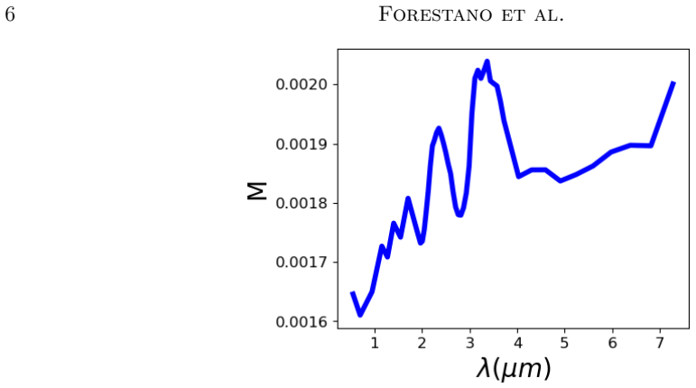
- [§6] Figure cross-references are inconsistent: 'Figure 6 depicts the original (blue dots) and the rebinned (red diamonds) spectra' should be Figure 7, and 'we reproduce in Figure 6' referring to the last row of Figure 12 should be Figure 8. Also 'the same exact 52 spectral wavelength values' is redundant.
- [§3.4 / Data Availability] The N M notation uses M_i and σ_i(M) for spectral mean and standard deviation, which can be confused with the spectrum M(λ). Consider renaming these features (e.g., μ_i, s_i). In addition, the manuscript provides no code or preprocessing scripts; only a link to the public ABC database is given, which is not sufficient to reproduce the exact 105,887-spectrum realization.
Circularity Check
No significant circularity: the ML benchmark is evaluated against held-out simulation labels and the WASP-39b case study is an external application; only minor non-load-bearing self-citations are present.
-
other
[Section 3.3, after Eq. (13)]
"It has been shown to be beneficial in practice during the Ariel Machine Learning Data Challenge (Yip et al. 2023; Unlu et al. 2023) and was theoretically motivated in Matchev et al. (2022b)."
This is a self-citation: the normalized-feature preprocessing that feeds the best-performing models is motivated by prior work by the same authors (Unlu et al. 2023 includes Forestano, Matchev, and Matcheva; Matchev et al. 2022b is by Matchev and Matcheva). However, the citation is not load-bearing: the paper independently benchmarks normalized versus standardized features on held-out TauREx spectra with known labels, so the ranking does not reduce to the cited prior work. Scored as a minor self-citation, not as a circular derivation.
full rationale
The central claim is a supervised regression benchmark: 52-bin TauREx spectra are the features and the generating atmospheric parameters are the targets, with 48,000 training and 12,000 test samples. Since test predictions are compared with known simulation truths, the reported XGB/SVM ranking is measured, not constructed by definition. The normalization and log-target preprocessing schemes are defined in the paper and compared across 48 configurations; the favorable result for normalization is empirically demonstrated, even though the choice is also motivated by self-citations. The WASP-39b case study is an out-of-sample application to real JWST data, and the literature values in Table 2 are not used as training labels, so the agreement is external validation rather than circular. The principal correctness caveat is that Section 3.4 describes a 'random subset of n=60,000 samples' split without grouping by the 5,900 unique planets from which the 105,887 spectra were generated; an instance-level split could permit the same planet's spectra in both train and test, inflating generalization estimates. That is a data-leakage/generalization risk, not a definitional equivalence or fitted-input-called-prediction circularity. Overall, the derivation is self-contained against external benchmarks, with only minor non-load-bearing self-citations, hence score 2.
Assumptions & free parameters
free parameters (1)
- Model hyperparameters (e.g., SVM C=500, gamma=0.028, epsilon=0.1; KNN k=6; RF n_estimators=115; XGB max_depth=6, learnin =
Values listed in Section 4.8; stated as 'optimized to achieve best performance'
assumptions (7)
- domain assumption TauREx3 forward model correctly simulates transmission spectra of hot Jupiters
- domain assumption Isothermal, 100-layer atmosphere with 1 Pa to 1e6 Pa pressure grid, He/H2=0.17, no clouds or hazes
- domain assumption Trace-gas abundances are independently sampled uniformly in log-space over fixed ranges (H2O 1e-9..1e-3, CO2 1e-9..1e-4, etc.)
- domain assumption Training on noiseless spectra is sufficient for models to perform on noisy real observations
- domain assumption The test distribution is representative; non-uniform planet/star sampling in the ABC database does not invalidate accuracy claims over the dynamical range
- domain assumption The rebinned WASP-39b spectrum is compatible with the 52-bin synthetic training features after normalization
- standard math scikit-learn and XGBoost implementations are correct
Cite this review
Pith. "Pith review of Supervised Machine Learning Methods with Uncertainty Quantification for Exoplanet Atmospheric Retrievals from Transmission Spectroscopy." pith.science (2026). https://pith.science/paper/IZ3OYGWM
@misc{pith2026250804982,
  author       = {Pith},
  title        = {Pith review of: Supervised Machine Learning Methods with Uncertainty Quantification for Exoplanet Atmospheric Retrievals from Transmission Spectroscopy},
  year         = {2026},
  howpublished = {\url{https://pith.science/paper/IZ3OYGWM}},
  note         = {Machine review of arXiv:2508.04982}
}
read the original abstract
Standard Bayesian retrievals for exoplanet atmospheric parameters from transmission spectroscopy, while well understood and widely used, are generally computationally expensive. In the era of the JWST and other upcoming observatories, machine learning approaches have emerged as viable alternatives that are both efficient and robust. In this paper we present a systematic study of several existing machine learning regression techniques and compare their performance for retrieving exoplanet atmospheric parameters from transmission spectra. We benchmark the performance of the different algorithms on the accuracy, precision, and speed. The regression methods tested here include partial least squares (PLS), support vector machines (SVM), k nearest neighbors (KNN), decision trees (DT), random forests (RF), voting (VOTE), stacking (STACK), and extreme gradient boosting (XGB). We also investigate the impact of different preprocessing methods of the training data on the model performance. We quantify the model uncertainties across the entire dynamical range of planetary parameters. The best performing combination of ML model and preprocessing scheme is validated on a the case study of JWST observation of WASP-39b.
Figures


Figures from the paper (23 more)


Reference graph
Works this paper leans on
-
[1]
Ahrer, E.-M., Stevenson, K. B., Mansfield, M., et al. 2023, Nature, 614, 653, 10.1038/s41586-022-05590-4
-
[2]
F., Changeat , Q., Waldmann , I
Al-Refaie , A. F., Changeat , Q., Waldmann , I. P., & Tinetti , G. 2021, , 917, 37, 10.3847/1538-4357/ac0252
-
[3]
Alderson, L., Wakeford, H. R., Alam, M. K., et al. 2023, Nature, 614, 664, 10.1038/s41586-022-05591-3
-
[4]
Ard \'e vol Mart \' nez , F., Min , M., Huppenkothen , D., Kamp , I., & Palmer , P. I. 2024, , 681, L14, 10.1051/0004-6361/202348367
-
[5]
Ardevol Martinez , F., Min , M., Kamp , I., & Palmer , P. I. 2022, arXiv e-prints, arXiv:2203.01236. 2203.01236
work page Pith review arXiv 2022
-
[6]
2023, arXiv e-prints, arXiv:2309.09337, 10.48550/arXiv.2309.09337
Aubin , M., Cuesta-Lazaro , C., Tregidga , E., et al. 2023, arXiv e-prints, arXiv:2309.09337, 10.48550/arXiv.2309.09337
-
[7]
2022, Nature Communications, 13, 2453, 10.1038/s41467-022-29939-5
Batzner, S., Musaelian, A., Sun, L., et al. 2022, Nature Communications, 13, 2453, 10.1038/s41467-022-29939-5
-
[8]
2012, The Astrophysical Journal, 753, 100, 10.1088/0004-637X/753/2/100
Benneke, B., & Seager, S. 2012, The Astrophysical Journal, 753, 100, 10.1088/0004-637X/753/2/100
Show all 85 references
-
[9]
Bishop, C. M. 2006, Pattern Recognition and Machine Learning (Information Science and Statistics) (Berlin, Heidelberg: Springer-Verlag)
2006
-
[10]
E., et al
Blecic , J., Harrington , J., Cubillos , P. E., et al. 2021, arXiv e-prints, arXiv:2104.12525. 2104.12525
2021 arXiv
-
[11]
A., & J., S
Breiman, L., Friedman, J., Olshen, R. A., & J., S. C. 1984, Classification and Regression Trees (1st ed.). (Chapman and Hall/CRC.), https://doi.org/10.1201/9781315139470
1984 doi
-
[12]
V., et al
Changeat , Q., Al-Refaie , A., Mugnai , L. V., et al. 2020, , 160, 80, 10.3847/1538-3881/ab9a53
2020 doi
-
[13]
Changeat , Q., & Yip , K. H. 2023, RAS Techniques and Instruments, 2, 45, 10.1093/rasti/rzad001
2023 doi
-
[14]
M., Latham , D
Charbonneau , D., Brown , T. M., Latham , D. W., & Mayor , M. 2000, , 529, L45, 10.1086/312457
2000 doi
-
[15]
2006, IEEE Transactions on Neural Networks, 17, 893, 10.1109/TNN.2006.875973
Chen, P.-H., Fan, R.-E., & Lin, C.-J. 2006, IEEE Transactions on Neural Networks, 17, 893, 10.1109/TNN.2006.875973
2006
-
[16]
Chen, T., & Guestrin, C. 2016, in Proceedings of the 22nd ACM SIGKDD International Conference on Knowledge Discovery and Data Mining, KDD '16 (New York, NY, USA: Association for Computing Machinery), 785–794, 10.1145/2939672.2939785
2016
-
[17]
D., Himes , M
Cobb , A. D., Himes , M. D., Soboczenski , F., et al. 2019, , 158, 33, 10.3847/1538-3881/ab2390
2019 doi
-
[18]
2023, The Astrophysical Journal Letters, 943, L10, 10.3847/2041-8213/acaead
Constantinou, S., Madhusudhan, N., & Gandhi, S. 2023, The Astrophysical Journal Letters, 943, L10, 10.3847/2041-8213/acaead
2023 doi
-
[19]
2013, The Astrophysical Journal, 768, 42, 10.1088/0004-637X/768/1/42
Cubillos, P., Harrington, J., Madhusudhan, N., et al. 2013, The Astrophysical Journal, 768, 42, 10.1088/0004-637X/768/1/42
2013 doi
-
[20]
E., Harrington , J., Blecic , J., et al
Cubillos , P. E., Harrington , J., Blecic , J., et al. 2021, arXiv e-prints, arXiv:2104.12524. 2104.12524
2021 arXiv
-
[21]
Dietterich, T. G. 1998, Neural Computation, 10, 1895, 10.1162/089976698300017197
1998 doi
-
[22]
2019 a , , 157, 242, 10.3847/1538-3881/ab1cb9
Edwards , B., Mugnai , L., Tinetti , G., Pascale , E., & Sarkar , S. 2019 a , , 157, 242, 10.3847/1538-3881/ab1cb9
2019 doi
-
[23]
2022, , 164, 15, 10.3847/1538-3881/ac6bf9
Edwards , B., & Tinetti , G. 2022, , 164, 15, 10.3847/1538-3881/ac6bf9
2022 doi
-
[24]
2019 b , Experimental Astronomy, 47, 29, 10.1007/s10686-018-9611-4
Edwards , B., Rice , M., Zingales , T., et al. 2019 b , Experimental Astronomy, 47, 29, 10.1007/s10686-018-9611-4
2019 doi
-
[25]
2022, , 658, A41, 10.1051/0004-6361/202141940
Falco , A., Zingales , T., Pluriel , W., & Leconte , J. 2022, , 658, A41, 10.1051/0004-6361/202141940
2022 doi
-
[26]
Fan, R.-E., Chen, P.-H., & Lin, C.-J. 2005, J. Mach. Learn. Res., 6, 1889–1918
2005
-
[27]
J., Kitzmann , D., et al
Fisher , C., Hoeijmakers , H. J., Kitzmann , D., et al. 2020, , 159, 192, 10.3847/1538-3881/ab7a92
2020 doi
-
[28]
T., Matchev, K
Forestano, R. T., Matchev, K. T., Matcheva, K., et al. 2023 a , Machine Learning: Science and Technology, 4, 025027, 10.1088/2632-2153/acd989
2023 doi
-
[29]
2023 b , Physics Letters B, 844, 10.1016/j.physletb.2023.138086
---. 2023 b , Physics Letters B, 844, 10.1016/j.physletb.2023.138086
2023
-
[30]
2023 c , Physics Letters B, 847, 138266, https://doi.org/10.1016/j.physletb.2023.138266
---. 2023 c , Physics Letters B, 847, 138266, https://doi.org/10.1016/j.physletb.2023.138266
2023
-
[31]
T., Matchev, K
Forestano, R. T., Matchev, K. T., Matcheva, K., & Unlu, E. B. 2023 d , The Astrophysical Journal, 958, 106, 10.3847/1538-4357/ad0047
2023 doi
-
[32]
2000, The Annals of Statistics, 28, 337 , 10.1214/aos/1016218223
Friedman, J., Hastie, T., & Tibshirani, R. 2000, The Annals of Statistics, 28, 337 , 10.1214/aos/1016218223
2000
-
[33]
2018, Monthly Notices of the Royal Astronomical Society, 474, 271–, https://doi.org/10.1093/mnras/stx2748
Gandhi, S., & Madhusudhan, N. 2018, Monthly Notices of the Royal Astronomical Society, 474, 271–, https://doi.org/10.1093/mnras/stx2748
2018 doi
-
[34]
E., Aronsson, J., Carlsson, O., et al
Gerken, J. E., Aronsson, J., Carlsson, O., et al. 2023, Artificial Intelligence Review, 56, 14605, 10.1007/s10462-023-10502-7
2023 doi
-
[35]
P., Line , M
Greene , T. P., Line , M. R., Montero , C., et al. 2016, , 817, 17, 10.3847/0004-637X/817/1/17
2016 doi
-
[36]
Griffith , C. A. 2014, Philosophical Transactions of the Royal Society of London Series A, 372, 20130086, 10.1098/rsta.2013.0086
2014
-
[37]
2020, , 160, 15, 10.3847/1538-3881/ab9176
Guzm \'a n-Mesa , A., Kitzmann , D., Fisher , C., et al. 2020, , 160, 15, 10.3847/1538-3881/ab9176
2020 doi
-
[38]
2023, , 672, A180, 10.1051/0004-6361/202243230
Haldemann , J., Ksoll , V., Walter , D., et al. 2023, , 672, A180, 10.1051/0004-6361/202243230
2023 doi
-
[39]
D., Cubillos , P
Harrington , J., Himes , M. D., Cubillos , P. E., et al. 2021, arXiv e-prints, arXiv:2104.12522. 2104.12522
2021
-
[40]
2001, The Elements of Statistical Learning, Springer Series in Statistics (New York, NY, USA: Springer New York Inc.)
Hastie, T., Tibshirani, R., & Friedman, J. 2001, The Elements of Statistical Learning, Springer Series in Statistics (New York, NY, USA: Springer New York Inc.)
2001
-
[41]
Hayes , J. J. C., Kerins , E., Awiphan , S., et al. 2020, , 494, 4492, 10.1093/mnras/staa978
2020 doi
-
[42]
2017, , 470, 2972, 10.1093/mnras/stx1453
Heng , K., & Kitzmann , D. 2017, , 470, 2972, 10.1093/mnras/stx1453
2017 doi
-
[43]
Hunter, J. D. 2007, Comput. Sci. Eng., 9, 90, 10.1109/MCSE.2007.55
2007 doi
-
[44]
Inc., P. T. 2015, Collaborative data science, Montreal, QC: Plotly Technologies Inc. https://plot.ly
2015
-
[45]
J., et al
Kirk , J., L \'o pez-Morales , M., Wheatley , P. J., et al. 2019, , 158, 144, 10.3847/1538-3881/ab397d
2019 doi
-
[46]
2020, , 890, 174, 10.3847/1538-4357/ab6d71
Kitzmann , D., Heng , K., Oreshenko , M., et al. 2020, , 890, 174, 10.3847/1538-4357/ab6d71
2020 doi
-
[47]
2016, in Positioning and Power in Academic Publishing: Players, Agents and Agendas, ed
Kluyver, T., Ragan-Kelley, B., P \'e rez, F., et al. 2016, in Positioning and Power in Academic Publishing: Players, Agents and Agendas, ed. F. Loizides & B. Scmidt (IOS Press), 87--90. https://eprints.soton.ac.uk/403913/
2016
-
[48]
Lim, L.-H., & Nelson, B. J. 2022, What is an equivariant neural network? 2205.07362
2022 arXiv
-
[49]
R., Wolf, A
Line, M. R., Wolf, A. S., Zhang, X., et al. 2013, The Astrophysical Journal, 775, 137, 10.1088/0004-637X/775/2/137
2013 doi
-
[50]
2025, , 984, L32, 10.3847/2041-8213/adc7aa
Lueber , A., Karchev , K., Fisher , C., et al. 2025, , 984, L32, 10.3847/2041-8213/adc7aa
2025 doi
-
[51]
J., & Lewis , N
MacDonald , R. J., & Lewis , N. K. 2022, , 929, 20, 10.3847/1538-4357/ac47fe
2022 doi
-
[52]
2018, Atmospheric Retrieval of Exoplanets, ed
Madhusudhan, N. 2018, Atmospheric Retrieval of Exoplanets, ed. H. J. Deeg & J. A. Belmonte (Cham: Springer International Publishing), 1--30, 10.1007/978-3-319-30648-3_104-1
2018 doi
-
[53]
2009, The Astrophysical Journal, 707, 24, 10.1088/0004-637X/707/1/24
Madhusudhan, N., & Seager, S. 2009, The Astrophysical Journal, 707, 24, 10.1088/0004-637X/707/1/24
2009 doi
-
[54]
2018, Nature Astronomy, 2, 719, 10.1038/s41550-018-0504-2
M \'a rquez-Neila , P., Fisher , C., Sznitman , R., & Heng , K. 2018, Nature Astronomy, 2, 719, 10.1038/s41550-018-0504-2
2018 doi
-
[55]
T., Matcheva , K., & Roman , A
Matchev , K. T., Matcheva , K., & Roman , A. 2022 a , The Planetary Sciences Journal, 3, 205, 10.3847/PSJ/ac880b
2022 doi
-
[56]
2022 b , , 939, 95, 10.3847/1538-4357/ac82f3
---. 2022 b , , 939, 95, 10.3847/1538-4357/ac82f3
2022 doi
-
[57]
2022 c , , 930, 33, 10.3847/1538-4357/ac610c
---. 2022 c , , 930, 33, 10.3847/1538-4357/ac610c
2022 doi
-
[58]
V., Pascale, E., Edwards, B., Papageorgiou, A., & Sarkar, S
Mugnai, L. V., Pascale, E., Edwards, B., Papageorgiou, A., & Sarkar, S. 2020, Experimental Astronomy, 50, 303–328, 10.1007/s10686-020-09676-7
2020 doi
-
[59]
C., & Madhusudhan , N
Nixon , M. C., & Madhusudhan , N. 2020, , 496, 269, 10.1093/mnras/staa1150
2020 doi
-
[60]
L., et al
Oreshenko, M., Lavie, B., Grimm, S. L., et al. 2017, The Astrophysical Journal Letters, 847, L3, 10.3847/2041-8213/aa8acf
2017 doi
-
[61]
2020, , 159, 6, 10.3847/1538-3881/ab5955
Oreshenko , M., Kitzmann , D., M \'a rquez-Neila , P., et al. 2020, , 159, 6, 10.3847/1538-3881/ab5955
2020 doi
-
[62]
2011, Journal of Machine Learning Research, 12, 2825
Pedregosa, F., Varoquaux, G., Gramfort, A., et al. 2011, Journal of Machine Learning Research, 12, 2825
2011
-
[63]
2023, Remote Sensing, 15, 635, 10.3390/rs15030635
Pluriel , W. 2023, Remote Sensing, 15, 635, 10.3390/rs15030635
2023 doi
-
[64]
2022, , 658, A42, 10.1051/0004-6361/202141943
Pluriel , W., Leconte , J., Parmentier , V., et al. 2022, , 658, A42, 10.1051/0004-6361/202141943
2022 doi
-
[65]
D., Lee, E
Powell, D., Feinstein, A. D., Lee, E. K. H., et al. 2024, Nature, 626, 979, 10.1038/s41586-024-07040-9
2024 doi
-
[66]
T., Matchev, K
Roman, A., Forestano, R. T., Matchev, K. T., Matcheva, K., & Unlu, E. B. 2023, Symmetry, 15, 10.3390/sym15071352
2023 doi
-
[67]
K., Mukherjee, S., et al
Rustamkulov, Z., Sing, D. K., Mukherjee, S., et al. 2023, Nature, 614, 659, 10.1038/s41586-022-05677-y
2023 doi
- [68]
-
[69]
D., O'Beirne , M
Soboczenski , F., Himes , M. D., O'Beirne , M. D., et al. 2018, arXiv e-prints, arXiv:1811.03390. 1811.03390
2018 arXiv
-
[70]
2021, arXiv e-prints, arXiv:2104.04824, 10.48550/arXiv.2104.04824
Tinetti , G., Eccleston , P., Haswell , C., et al. 2021, arXiv e-prints, arXiv:2104.04824, 10.48550/arXiv.2104.04824
2021 doi
-
[71]
Trevor Hastie, Robert Tibshirani, J. F. 2009, The Elements of Statistical Learning (New York, New York: Springer)
2009
-
[72]
P., Zingales , T., et al
Tsiaras , A., Waldmann , I. P., Zingales , T., et al. 2018, The Astronomical Journal, 155, 156, 10.3847/1538-3881/aaaf75
2018 doi
-
[73]
B., Forestano, R
Unlu, E. B., Forestano, R. T., Matchev, K. T., & Matcheva, K. 2023, Reproducing Bayesian Posterior Distributions for Exoplanet Atmospheric Parameter Retrievals with a Machine Learning Surrogate Model. 2310.10521
2023 arXiv
-
[74]
C., & Varoquaux, G
van der Walt, S., Colbert, S. C., & Varoquaux, G. 2011, Computing in Science Engineering, 13, 22, 10.1109/MCSE.2011.37
2011 doi
-
[75]
E., et al
Virtanen, P., Gommers, R., Oliphant, T. E., et al. 2020, Nature Methods, 17, 261, 10.1038/s41592-019-0686-2
2020 doi
-
[76]
Waldmann , I. P. 2016, , 820, 107, 10.3847/0004-637X/820/2/107
2016 doi
-
[77]
P., Tinetti, G., Rocchetto, M., et al
Waldmann, I. P., Tinetti, G., Rocchetto, M., et al. 2015, The Astrophysical Journal, 802, 107, 10.1088/0004-637X/802/2/107
2015 doi
-
[78]
2000, Technical report
Wegelin, J. 2000, Technical report
2000
-
[79]
2021, , 913, 114, 10.3847/1538-4357/abee94
Welbanks , L., & Madhusudhan , N. 2021, , 913, 114, 10.3847/1538-4357/abee94
2021 doi
- [80]
-
[81]
H., Changeat , Q., Al-Refaie , A., & Waldmann , I
Yip , K. H., Changeat , Q., Al-Refaie , A., & Waldmann , I. P. 2024, , 961, 30, 10.3847/1538-4357/ad063f
2024 doi
-
[82]
H., Changeat, Q., Nikolaou, N., et al
Yip, K. H., Changeat, Q., Nikolaou, N., et al. 2021, The Astronomical Journal, 162, 195, 10.3847/1538-3881/ac1744
2021 doi
-
[83]
H., Waldmann , I
Yip , K. H., Waldmann , I. P., Changeat , Q., et al. 2022, arXiv e-prints, arXiv:2206.14642. 2206.14642
2022 arXiv
-
[84]
H., Changeat, Q., Waldmann, I., et al
Yip, K. H., Changeat, Q., Waldmann, I., et al. 2023, Proceedings of Machine Learning Research, 220, 1. https://proceedings.mlr.press/v220/yip23a.html
2023
-
[85]
Zingales , T., & Waldmann , I. P. 2018, , 156, 268, 10.3847/1538-3881/aae77c
2018 doi
Reviewed August 5, 2026 · model on record in the stance chip above.
Discussion (0). Sign in to comment.