REVIEW 3 major objections 4 minor 2 cited by
Sparse but Wrong: Incorrect L0 Leads to Incorrect Features in Sparse Autoencoders
T0 review · 3 major / 4 minor · reviewed 2026-08-05 · deepseek-v4-flash
Pith's one-line read Setting an SAE's sparsity (L0) too low or too high makes it mix correlated features instead of isolating them, and a new decoder-projection metric can find the correct setting.
desk verdict The toy-model result is real and worth keeping — low-L0 SAEs beat the ground-truth dictionary on MSE — but the LLM-side 'correct L0' is a visual elbow, not a formal optimum, so 'most SAEs are too sparse' is plausible, not proven. read the letter →
The pith
A machine-rendered reading of the paper's core claim, the machinery that carries it, and where it could break.
The reading
What carries the argument
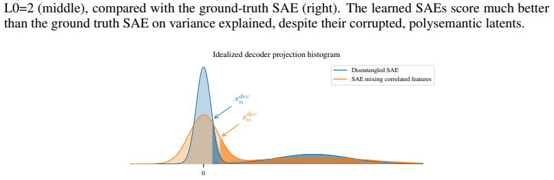
Nth decoder projection score (s_dec_n): compute projections of (x − b_dec) onto each decoder column for a batch, sort all values, and take the nth-highest (with n below h/2). At the correct L0, most non-firing latents have near-zero projection on arbitrary inputs, while mixed latents project strongly, so a low s_dec_n signals monosemanticity. The companion object is the toy model itself: orthogonal feature directions with correlated Bernoulli firing, in which the true L0 is known and the ground-truth SAE can be constructed, providing the controlled demonstration that low-L0 SAEs are driven by MSE to hedge correlated features.
What would settle it
Run the paper's toy-model experiment with L0 below the true L0 but with the feature correlation matrix modified so that correlated features never co-occur in the same training sample; the claim predicts latents stop mixing, since the reconstruction incentive to hedge disappears. Separately, on a layer not studied in the paper, sweep L0 and compare the s_dec_n elbow with k-sparse probing F1: divergence much larger than the alignment shown for Gemma-2-2b and Llama-3.2-1b would falsify the metric's general validity.
Extended reading notes
Core claim
Working from the Linear Representation Hypothesis, the paper builds toy models with known orthogonal features whose firing is correlated, so the true L0 is known. It shows that when the SAE's L0 is below the true value, the reconstruction loss rewards latents that absorb positive components of positively correlated features and negative components of anti-correlated ones; a deliberately corrupted SAE beats the ground-truth dictionary on variance explained. When L0 is too high, the SAE converges to degenerate mixed solutions. The paper introduces s_dec_n, the nth-highest projection of decoder directions onto training activations, which is minimized at the true L0 in toy models and whose elbow
Load-bearing premise
The toy model—orthogonal feature directions firing via a correlated Bernoulli process—is assumed to capture enough of how real LLM features behave that the low-L0 mixing mechanism and the s_dec_n minimum transfer to actual models; the paper validates this on only two small LLMs and a few layers, and explicitly leaves non-linear features (Appendix A.8) out of scope.
Editorial extensions
If this is right
- Most open-source SAEs have L0 below 100 while the paper's proxy points to roughly 200–250 for Gemma-2-2b layer 12; if the claim holds, widely used feature dictionaries are partially mixed and noisier than reported.
- Sparsity–reconstruction tradeoff plots should not be the primary SAE evaluation: they can rank a feature-mixing SAE above a perfect one.
- Practitioners should sweep L0 and select it with s_dec_n or decoder pairwise cosine similarity, rather than treating sparsity as a free choice.
- JumpReLU SAEs tolerate high L0 better than BatchTopK SAEs because per-latent thresholds adapt and "stick" near the correct firing rate.
- Starting training with L0 too low can permanently trap the SAE in a bad local minimum, so L0 schedules should approach the target from above.
Reading between the lines
- If the mixing mechanism transfers, a concrete fingerprint of too-low L0 in real SAEs is latents carrying negative components of anti-correlated features; inspecting latents for topically unrelated concepts (the paper's 'French poetry' vs 'Harry Potter' example) is a testable diagnostic.
- The argument implies that any sparse dictionary learner on correlated data—not just LLM SAEs—has a data-dependent correct sparsity, so similar decoder-projection diagnostics may transfer to other sparse coding settings.
- Because the appendix shows low-L0 damage is hard to reverse, automatic L0 search should be built as a high-to-low annealing; the paper's own heuristic embodies this but it is not stated as a general design principle.
- The metric's stable elbow across small models suggests a cheaper validation protocol: train a small SAE suite on a few layers, locate the elbow, and extrapolate L0 for the full suite—an extension the paper does not claim.
Editorial analysis
A structured set of objections, weighed in public.
Referee Report
Summary. The paper argues that the L0 sparsity level of a sparse autoencoder is not a free hyperparameter but has a correct value determined by the underlying data. Using toy models with ground-truth correlated features, it shows that when L0 is set too low, SAEs mix positively and negatively correlated features to improve reconstruction, and when L0 is set too high, they find degenerate mixed solutions. The authors propose an nth-decoder-projection metric, s_dec_n, that is minimized at the true L0 in toy models, and they report that an 'elbow' in this metric in LLM SAEs (Gemma-2-2b, Llama-3.2-1b) coincides with peak k=16 sparse probing performance. They conclude that most publicly available SAEs are trained with L0 too low and that sparsity–reconstruction tradeoff plots are misleading.
Significance. If the central claim holds, the paper would be a useful corrective to the common practice of treating L0 as a purely neutral axis in an evaluation tradeoff. The toy experiments are well-controlled: they use known ground truth, multiple seeds, and explicit comparison of learned SAEs against a ground-truth SAE, and the demonstration that a lower-MSE SAE can have less monosemantic latents is concrete and reproducible. The authors also ship code and, in the appendices, honestly document where their metric does not behave cleanly. The most valuable contribution is the identification of feature-mixing as a failure mode of low-L0 SAEs and the empirical warning that sparsity–reconstruction plots can reward incorrect solutions. However, the LLM-side validation of the proposed metric is not yet established, and the broad practical claim about public SAEs rests on that validation.
major comments (3)
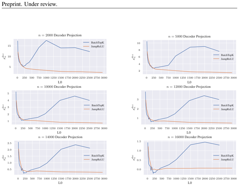
- [§4, Fig. 9; Appendix A.9] The LLM 'correct L0' is read from a visual elbow, not from a defined optimum. For Gemma-2-2b layer 5, Figure 9 shows that the global minimum of s_dec_n lies in the shallow high-L0 region (roughly L0≈750–1000), not at the claimed L0≈200. Appendix A.9 explicitly states that 'These plots never have a clear global minimum at the “elbow” point, but the “elbow” is always at the same point regardless of choice of N.' This undercuts the abstract's claim that the method 'finds the correct L0' in LLM SAEs. Because the same s_dec_n elbow is later used to conclude that public SAEs with L0<100 are too low, the LLM validation is circular unless the elbow is replaced by a precise, reproducible criterion and shown to be the relevant optimum of a well-defined objective. The independent k=16 sparse-probing peak helps, but then the metric is not what identifies the L0; the probing benchmark is.
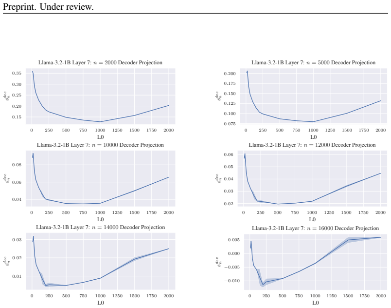
- [§3.5, Eq. (5); §4 and Figs. 17–19] The metric depends on a free hyperparameter n, and the LLM results are not robust to that choice. In the paper, n=16k (about h/2) is selected after inspecting the curves; for Gemma-2-2b layer 12 JumpReLU SAEs, only n=16k gives a clear s_dec_n minimum at the claimed 200–250, while other n values do not. For Gemma-2-2b layer 5, no n gives a global minimum at the elbow. A method whose output changes qualitatively with an unspecified hyperparameter needs either a principled way to choose n or a sensitivity analysis demonstrating the conclusion is invariant. As written, the toy-model result (n=12 and n=18 both minimized at the true L0) does not transfer to the LLM setting, so the claim that s_dec_n can 'guide the search for the correct L0' is not supported by the LLM experiments.
- [§6 and §A.8] The broad practical conclusion that 'most commonly used SAEs have an L0 that is too low' is based on two small LLMs (Gemma-2-2b, Llama-3.2-1b) and a few layers, with the toy model restricted to orthogonal linear features and correlated Bernoulli firing. Appendix A.8 acknowledges the non-linear feature exclusion and the limited layer coverage, but the Discussion and abstract do not temper the conclusion accordingly. This is not an internal inconsistency, but it means the headline claim is considerably stronger than the empirical support. The authors should either add evidence across more models/layers or explicitly reframe the claim as a hypothesis to be tested in broader settings.
minor comments (4)
- [Throughout] Typographical issues: 'monsemanticity' in the Figure 1 caption should be 'monosemanticity'; 'afterall' should be 'after all'; 'saes' should be 'SAEs'; 'n th' in Section 3.5 should be 'nth'.
- [Fig. 6] The idealized histogram contains unrendered text ('0 sdec n sdec n'), which makes the figure hard to interpret. Please clean up the labels.
- [Fig. 7 and Appendix A.6] The hyperparameter is sometimes called n and sometimes N; the caption of Figure 7 says 'slopes ... depend on N' while the text uses n. Please standardize.
- [§3.5] The rationale for choosing n 'sufficiently larger than a reasonable guess at the correct L0' is vague. A more formal statement—e.g., in terms of the expected number of active latents above a projection threshold—would help practitioners implement the metric.
Circularity Check
No significant circularity: toy ground truth anchors the central claim; the LLM 'elbow' heuristic is a validity concern, not a circular reduction.
full rationale
The paper's central mechanism—that setting L0 too low causes SAEs to mix correlated features—is established in a synthetic toy model with externally known ground-truth features and true L0. The SAEs are trained from a ground-truth initialization, and the MSE comparison directly demonstrates the incentive to mix features (Section 3.3). This does not reduce to the paper's proposed metric or to any fitted parameter. The s_dec_n metric is first validated against the known true L0 in the toy model (Section 3.5), and in LLM experiments it is compared to an independent external benchmark, sparse probing from Kantamneni et al. (2025). The paper explicitly acknowledges that the LLM s_dec_n curves do not always have a global minimum at the claimed L0, instead invoking a visually defined 'elbow' (Section 4, Appendix A.9). This weakens the LLM validation and raises a legitimate robustness concern, but it is not circular: the elbow location is reported as coinciding with peak sparse probing, not fitted to it by construction. The self-citations to Chanin et al. (2025) feature hedging and SAELens are contextual and not load-bearing; the toy experiments stand on their own. No uniqueness theorem is imported from prior work, and no ansatz is smuggled in solely via citation. Therefore the derivation chain is not circular, though the LLM-based 'correct L0' claims are less well-supported than the toy-model results.
Assumptions & free parameters
free parameters (3)
- n (rank index for s_dec_n) =
12 and 18 in toy; 2000 to 16000 in LLM; best near h/2
- toy model correlation matrix C =
specified in Fig 11 for large toy; 5-feature structure in Sec 3.1
- feature firing probabilities p_i =
p=0.4 for small toy; 0.345 down to 0.05 for large toy
assumptions (4)
- domain assumption LLM features are approximately orthogonal linear directions and activations are sums of active feature vectors (Linear Representation Hypothesis).
- ad hoc to paper For a correctly set L0, inactive latents have near-zero decoder projections, and feature mixing monotonically increases the nth decoder projection, so s_dec_n is minimized at the true L0.
- domain assumption Sparse probing performance is a valid proxy for SAE feature correctness in LLMs.
- domain assumption The implemented BatchTopK and JumpReLU losses (including the JumpReLU pseudo-gradient) match SOTA training procedures.
Cite this review
Pith. "Pith review of Sparse but Wrong: Incorrect L0 Leads to Incorrect Features in Sparse Autoencoders." pith.science (2026). https://pith.science/paper/RDIJREXQ
@misc{pith2026250816560,
  author       = {Pith},
  title        = {Pith review of: Sparse but Wrong: Incorrect L0 Leads to Incorrect Features in Sparse Autoencoders},
  year         = {2026},
  howpublished = {\url{https://pith.science/paper/RDIJREXQ}},
  note         = {Machine review of arXiv:2508.16560}
}
read the original abstract
Sparse Autoencoders (SAEs) extract features from LLM internal activations, meant to correspond to interpretable concepts. A core SAE training hyperparameter is L0: how many SAE features should fire per token on average. Existing work compares SAE algorithms using sparsity-reconstruction tradeoff plots, implying L0 is a free parameter with no inherently correct value aside from its effect on reconstruction. In this work we study the effect of L0 on SAEs, and show that if L0 is not set correctly, the SAE fails to disentangle the underlying features of the LLM. If L0 is too low, the SAE will mix correlated features to improve reconstruction. If L0 is too high, the SAE finds degenerate solutions that also mix features. Further, we present a proxy metric that can help guide the search for the correct L0 for an SAE on a given training distribution. We show that our method finds the correct L0 in toy models and coincides with peak sparse probing performance in LLM SAEs. We find that most commonly used SAEs have an L0 that is too low. Our work shows that practitioners must set L0 correctly to train SAEs with monosemantic features.
Figures


Figures from the paper (19 more)






Forward citations
Cited by 2 Pith papers
-
Perplexity Can Miss SAE Feature Damage Under Quantization
Quantization of LLMs can degrade many SAE features even when perplexity improves or stays similar, as shown by correlation measurements on frozen SAEs for Pythia-70M and Gemma-2-2B models across INT8 to INT4.
-
SATORI: Static Test Oracle Generation for REST APIs
SATORI statically infers REST API test oracles from OpenAPI specs via LLMs, reporting F1 74.3%, above AGORA+'s 69.3%, with 18 confirmed bugs; the supplied full text, however, is a different paper.
Reference graph
Works this paper leans on
-
[4]
David Chanin, Tom´aˇs Dulka, and Adri`a Garriga-Alonso. Feature hedging: Correlated features break narrow sparse autoencoders.arXiv preprint arXiv:2505.11756,
-
[5]
Dictionary learning optimization techniques.https: //transformer-circuits.pub/2025/january-update,
Tom Conerly, Hoagy Cunningham, Adly Templeton, Jack Lindsey, Basil Hos- mer, and Adam Jermyn. Dictionary learning optimization techniques.https: //transformer-circuits.pub/2025/january-update,
work page 2025
-
[6]
URLhttps://arxiv.org/abs/2407.21783. Nelson Elhage, Tristan Hume, Catherine Olsson, Nicholas Schiefer, Tom Henighan, Shauna Kravec, Zac Hatfield-Dodds, Robert Lasenby, Dawn Drain, Carol Chen, et al. Toy models of superposi- tion.arXiv preprint arXiv:2209.10652,
-
[8]
URLhttps://openreview.net/forum?id=d63a4AM4hb. Leo Gao, Stella Biderman, Sid Black, Laurence Golding, Travis Hoppe, Charles Foster, Jason Phang, Horace He, Anish Thite, Noa Nabeshima, Shawn Presser, and Connor Leahy. The Pile: An 800gb dataset of diverse text for language modeling.arXiv preprint arXiv:2101.00027,
-
[10]
Are sparse autoencoders useful? a case study in sparse probing.arXiv preprint arXiv:2502.16681,
Subhash Kantamneni, Joshua Engels, Senthooran Rajamanoharan, Max Tegmark, and Neel Nanda. Are sparse autoencoders useful? a case study in sparse probing.arXiv preprint arXiv:2502.16681,
-
[11]
Adam: A method for stochastic optimization.arXiv preprint arXiv:1412.6980,
Diederik P Kingma and Jimmy Ba. Adam: A method for stochastic optimization.arXiv preprint arXiv:1412.6980,
-
[12]
URLhttps://openreview.net/forum?id=UGpGkLzwpP. Senthooran Rajamanoharan, Tom Lieberum, Nicolas Sonnerat, Arthur Conmy, Vikrant Varma, J´anos Kram´ar, and Neel Nanda. Jumping ahead: Improving reconstruction fidelity with jumprelu sparse autoencoders.arXiv preprint arXiv:2407.14435,
-
[13]
URLhttps://arxiv.org/abs/2408.00118. Demian Till. Do sparse autoencoders find true features?LessWrong,
Show all 23 references
-
[14]
Zhengxuan Wu, Aryaman Arora, Atticus Geiger, Zheng Wang, Jing Huang, Dan Jurafsky, Christo- pher D Manning, and Christopher Potts
URLhttps://www.lesswrong.com/posts/QoR8noAB3Mp2KBA4B/ do-sparse-autoencoders-find-true-features. Zhengxuan Wu, Aryaman Arora, Atticus Geiger, Zheng Wang, Jing Huang, Dan Jurafsky, Christo- pher D Manning, and Christopher Potts. Axbench: Steering llms? even simple baselines out...
-
[15]
A APPENDIX A.1 SAETRAINING ARCHITECTURE DEFINITIONS In this work we focus on JumpReLU (Conerly et al., 2025; Rajamanoharan et al.,
2025
-
[16]
For BatchTopK SAEs, there is no sparsity penalty as sparsity is enforced by the BatchTopK function
SAEs. For BatchTopK SAEs, there is no sparsity penalty as sparsity is enforced by the BatchTopK function. The auxiliary lossL P for BatchTopK is as follows, wheree is the SAE training error residual, andˆeis a reconstruction using the topk aux dead latents (meaning the latents...
2025
-
[17]
We use a learning rate of3e −4 with no warmup or decay
A.3 LLM SAETRAINING DETAILS For BatchTopK SAEs, we ensure that the decoder remains normalized with||W dec||2 = 1sos dec n calculations use the same scale for every latent. We use a learning rate of3e −4 with no warmup or decay. For JumpReLU SAEs, we broadly follow the training...
2025
-
[18]
The metric is minimized at the true L0
The shaded area is 1 stdev. The metric is minimized at the true L0. 0 250 500 750 1000 1250 1500 1750 2000 L0 0.008 0.010 0.012 0.014 Cosine Similarity Decoder Pairwise Cosine Similarity 0 250 500 750 1000 1250 1500 1750 2000 L0 0.78 0.80 0.82 F1 Score k=16 Sparse Probing Gemm...
2000
-
[19]
We include all SAEs cross-listed in both SAELens and Neuronpedia with an L0 reported in SAELens
and SAELens (Bloom et al., 2024). We include all SAEs cross-listed in both SAELens and Neuronpedia with an L0 reported in SAELens. We show the results as a histogram in Figure
2024
-
[20]
However, we find that most open-source SAEs have L0 below 100, much lower than our analysis expects to be ideal
Our analysis shows that for layer 12 of Gemma-2-2b, the correct L0 should be around 200-250. However, we find that most open-source SAEs have L0 below 100, much lower than our analysis expects to be ideal. A.8 LIMITATIONS We limited the scope of our investigation to features s...
2025
-
[21]
elbow” point, but the “elbow
We note that in all cases, low L0 behavior is similar: no matter the value of N,s dec n increases dramatically at low L0. However, the high L0 behavior is less consistent. We always see a similar “elbow” in the plots at roughly the same place regardless of N, but sometimes thi...
2000
-
[22]
We see that BatchTopK SAEs rely much more heavily on the encoder bias than JumpReLU SAEs seem to, with a much wider variance in values and a sharper decrease compared to JumpReLU. We expect this is because BatchTopK cannot coordinate the cutoff threshold with the encoder direc...
2000
-
[23]
The threshold for BatchTopK is much higher than it is for JumpReLU, and the threshold decreases as L0 increses
Here as well, we see dramatic differences between BatchTopK and JumpReLU SAEs. The threshold for BatchTopK is much higher than it is for JumpReLU, and the threshold decreases as L0 increses. This makes sense, since using a lower cutoff means more latents can fire. However, Jum...
2000
-
[2020]
Scaling and evaluating sparse autoencoders.arXiv preprint arXiv:2406.04093,
Leo Gao, Tom Dupr ´e la Tour, Henk Tillman, Gabriel Goh, Rajan Troll, Alec Radford, Ilya Sutskever, Jan Leike, and Jeffrey Wu. Scaling and evaluating sparse autoencoders.arXiv preprint arXiv:2406.04093,
-
[2022]
Decomposing the dark matter of sparse autoen- coders.arXiv preprint arXiv:2410.14670,
Joshua Engels, Logan Riggs, and Max Tegmark. Decomposing the dark matter of sparse autoen- coders.arXiv preprint arXiv:2410.14670,
-
[2023]
Batchtopk sparse autoencoders.arXiv preprint arXiv:2412.06410,
Bart Bussmann, Patrick Leask, and Neel Nanda. Batchtopk sparse autoencoders.arXiv preprint arXiv:2412.06410,
-
[2024]
Learning multi-level features with matryoshka sparse autoencoders.arXiv preprint arXiv:2503.17547,
Bart Bussmann, Noa Nabeshima, Adam Karvonen, and Neel Nanda. Learning multi-level features with matryoshka sparse autoencoders.arXiv preprint arXiv:2503.17547,
-
[2025]
A is for absorption: Studying feature splitting and absorption in sparse autoencoders.arXiv preprint arXiv:2409.14507,
David Chanin, James Wilken-Smith, Tom ´aˇs Dulka, Hardik Bhatnagar, and Joseph Bloom. A is for absorption: Studying feature splitting and absorption in sparse autoencoders.arXiv preprint arXiv:2409.14507,
Reviewed August 5, 2026 · model on record in the stance chip above.
Discussion (0). Sign in to comment.