REVIEW 3 major objections 5 minor 7 cited by
Two JWST epochs reveal 465 variable galactic nuclei in one field, while Little Red Dots stay quiet.
Reviewed by Pith at T0; open to challenge. T0 means a machine referee read the full paper against a public rubric. the ladder, T0–T4 →
T0 review · deepseek-v4-flash
2026-08-04 15:20 UTC pith:6D3HCW2Y
load-bearing objection Solid NEXUS variability catalog and slightly tighter LRD upper limits, but the self-calibrated noise curve deserves scrutiny before the 465 and 3-10% numbers are taken at face value. the 3 major comments →
NEXUS: A Search for Nuclear Variability with the First Two JWST NIRCam Epochs
The pith
A machine-rendered reading of the paper's core claim, the machinery that carries it, and where it could break.
Core claim
Using the first two NEXUS epochs (September 2024 and June 2025), the authors match the point-spread function between the two epochs with SFFT and direct subtraction, and adopt the smaller of the two measured magnitude changes as the fiducial value per source. From the 3σ-clipped scatter of this Δm against source magnitude they construct a noise floor, debias the measurements, and select 465 sources whose flux change exceeds 3σ of that floor and survives visual inspection. These variable sources follow the same photometric redshift distribution as the parent sample, indicating they are mostly distant AGNs. Separately, the ten spectroscopically confirmed broad-line Little Red Dots in the field
What carries the argument
The central mechanism is difference imaging with two independent subtractions: SFFT, which models spatial PSF variations and differential background in the Fourier domain, and direct frame subtraction. The 'BEST' measurement combines them by taking the smaller Δm per source. A smooth σ_Δm(m) curve, built from the 3σ-clipped scatter of the same Δm data under the assumption that most sources are non-variable, serves as the noise floor for defining >3σ variability and for setting upper limits on Little Red Dot variability.
Load-bearing premise
The noise curve that sets the 3σ threshold and the Little Red Dot upper limits is measured from the scatter of the same Δm data under the assumption that most sources in each magnitude bin are non-variable; if correlated image-subtraction systematics or a large population of real variables inflate that scatter, both the 465-source catalog and the LRD limits shift.
What would settle it
Compute the Δm scatter on blank sky positions with the same difference-imaging pipeline; if blank-sky noise alone reproduces the σ_Δm(m) curve, the variable-source threshold is noise-limited, while if source positions show excess scatter the curve is contaminated. Alternatively, a third epoch at ~2-month cadence should confirm a large fraction of the 465 candidates as same-sense repeaters; a low repetition fraction would indicate systematics dominated the selection.
If this is right
- The 465-source catalog provides immediate targets for spectroscopy; the majority should confirm as broad-line AGNs, with a minority possibly being tidal disruption events or supernovae.
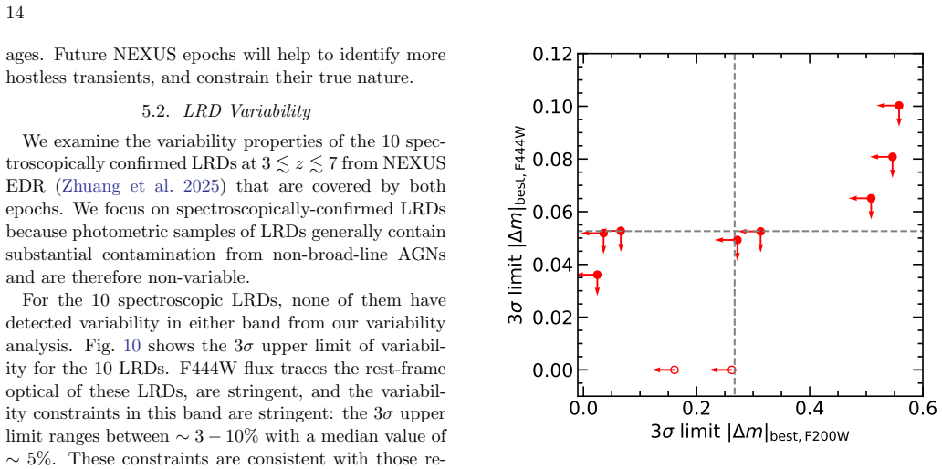
- The 3-10% (median ~5%) F444W non-variability of the ten Little Red Dots constrains models in which the rest-frame optical continuum arises from an extended photosphere or scattered light, both of which smooth variability.
- Difference imaging cuts the scatter in measured flux changes by more than 30% compared with single-epoch aperture photometry, making it the preferred method for variability searches in future JWST monitoring programs.
- As NEXUS continues with a 2-month cadence through 2028, the bright subset (F444W < 26) of these variables will become high-priority targets for NIRSpec/MSA spectroscopy to establish their nature.
- The 465 variables include extreme cases with |Δm| > 1 and off-nucleus flux changes, which are promising candidates for rare nuclear transients and supernovae that can be confirmed with continued monitoring.
Where Pith is reading between the lines
- If the Little Red Dot non-variability persists across the full 18-epoch Deep cadence, it would argue that their rest-frame optical continuum is produced by a spatially extended or self-regulated region rather than a compact, unobscured accretion disk.
- The same difference-imaging pipeline could be applied to other multi-epoch JWST Treasury fields, and the >30% sensitivity gain over epoch photometry is a directly transferable result for building a uniform census of nuclear variability.
- With only two epochs, the brightening-versus-dimming asymmetry at faint magnitudes could be used as a statistical flag for transient candidates before spectra arrive; a third epoch will reveal whether the 465 sources repeat in the same sense or represent stochastic AGN flickering.
- The LRD upper limits, being set on a 9-month observed baseline, correspond to rest-frame time scales of roughly 1-2 months at z~3-7; extending the baseline to several years will probe whether low-level variability appears on longer rest-frame time scales.
Editorial analysis
A structured set of objections, weighed in public.
Referee Report
Summary. This paper presents a two-epoch JWST/NIRCam variability search over ~25,000 NEXUS sources in F200W and F444W, using difference imaging via direct frame subtraction and the SFFT algorithm. The authors adopt the smaller absolute magnitude change from the two subtraction methods as the fiducial 'BEST' measurement, define variability by |Δm_debiased| > 3σ_Δm, where σ_Δm is a magnitude-dependent noise curve fitted to the 3σ-clipped scatter of the same Δm_BEST data, and after visual inspection produce a catalog of 465 high-confidence variable sources. They also analyze ten spectroscopically confirmed broad-line Little Red Dots, report no significant variability, and derive 3σ F444W upper limits of roughly 3–10% (median ~5%). The paper argues that these limits imply weak rest-frame optical continuum variability in LRDs.
Significance. If the statistical calibration is sound, this is a valuable contribution: it demonstrates the power of NIRCam difference imaging for detecting low-level nuclear variability, provides a public catalog of variable sources at high redshift, and places important constraints on LRD accretion models. The detailed description of the SFFT subtraction pipeline and the careful comparison of methods are strengths. However, the central claims—the 465-source catalog and the quantitative LRD upper limits—rely on a self-calibrated noise curve whose statistical meaning is not well established, so the current version overstates the robustness of the reported thresholds.
major comments (3)
- [Section 4, Fig. 7] The variability threshold is calibrated from the same Δm_BEST distribution used for selection. Δm_BEST is the smaller |Δm| of SFFT and direct subtraction; for non-variable sources this is the minimum of two positive-valued noise realizations, which has a narrower, non-Gaussian distribution than the underlying per-method noise. Hence 3σ_Δm does not correspond to a 3σ detection in the original measurement. The initial candidate fraction (~3%) is an order of magnitude higher than the ~0.3% expected for 3σ Gaussian noise, and 36% of candidates are later rejected by visual inspection—both consistent with an underestimated noise floor. The same σ_Δm curve feeds the LRD upper limits in Section 5.2. Please provide an independent noise calibration (e.g., from the scatter of repeated noise realizations, the difference between the two subtraction methods on known non-variables, or injected sources)
- [Section 3.4, Eq. (1)] The 'BEST' metric, min(|Δm|) of the two methods, introduces a systematic bias in the measured amplitude for real variables (pulling them toward zero) and is not a standard self-consistent statistic. Its distribution is method-dependent and non-Gaussian, so thresholds based on its clipped standard deviation are not transferable to statements about individual-source significance. This affects both the variable catalog and the upper limits. The authors should either combine the two measurements with a statistically motivated estimator (e.g., inverse-variance weighting after due error calibration) or apply separate thresholds for each method, and should characterize the bias using simulations of injected variability.
- [Section 5.2, Fig. 10] The LRD F444W upper limits are directly read off the self-calibrated σ_Δm curve. Given the above calibration concerns, these are not true 3σ upper limits; a factor of 1.5–2 underestimate in the noise would shift the median limit from ~5% toward ~8–10%, weakening the quantitative claim. Also, the text says 'ten LRDs' but Fig. 10 marks two objects without F444W measurements; the authors should explicitly state that only 8 LRDs contribute to the F444W median and clarify the impact on the quoted range.
minor comments (5)
- [Section 3.4] The text says 'we adopt the smaller Δm value' but the analysis and figures clearly use the smaller |Δm|. Please use the unambiguous notation throughout.
- [Section 4] The threshold for switching from a straight-line fit to a fourth-order polynomial in the σ_Δm(m) curve is not specified. State the magnitude break and its rationale.
- [Figure 10] The caption should explain why two LRD sources have no F444W measurements (e.g., outside the F444W coverage or other reasons).
- [Section 5.2] When comparing with Kokubo & Harikane (2024) and Zhang et al. (2025), include the quoted limits from those works to make the stated consistency and 'somewhat tighter' claim quantitative.
- [Table 1] The table format is dense and the repetition of columns for four methods/apertures may hamper usability. Consider providing a separate machine-readable table with a simplified schema, and point to its column descriptions in the README.
Circularity Check
No significant circularity: variability thresholds are empirical noise calibrations, not derived predictions.
full rationale
The paper's central claims are empirical measurements: a catalog of 465 variable sources and 3σ upper limits on LRD variability. The σ_Δm(m) noise curve used for thresholding is fit to the same Δm_BEST data under the explicit assumption that most sources are non-variable (Section 4). This is a standard self-calibration of the noise model, not a circular derivation. The variable selection is defined as |Δm_debiased| > 3σ_Δm, so the curve acts as a significance threshold; the selected sources are outliers relative to the fitted scatter, and 36% are rejected by independent visual inspection. The LRD upper limits are 3σ_Δm values at the LRD magnitudes, i.e., noise-based upper limits, not predictions derived from the fitted parameters. No equation is defined in terms of the result it is supposed to produce, and no fitted constant is renamed as a prediction. Self-citations to NEXUS EDR/overview papers and the LRD spectroscopy paper (Zhuang et al. 2024, 2025; Shen et al. 2024) are data provenance and sample definition, not load-bearing circular arguments. Any concern that the clipped scatter underestimates correlated systematics is a correctness/robustness issue, not a circularity issue. Therefore the derivation chain is self-contained and non-circular.
Axiom & Free-Parameter Ledger
free parameters (3)
- sigma_Delta-m(m) noise-curve coefficients =
not quoted in draft
- SFFT masking thresholds =
FLUX_APER = 30, 45, 150 microJy; CLASS_STAR = 0.98, 0.9, 0.7
- SFFT algorithm hyperparameters =
kernel half-widths 11 px F200W and 5 px F444W; 3x3 and 6x6 B-spline knot grids; Tikhonov lambda = 3e-5; first-order phot
axioms (4)
- domain assumption The majority of sources in each magnitude bin are non-variable, so the 3-sigma-clipped scatter of Delta-m equals the measurement noise floor.
- domain assumption Residual PSF-matching and background artifacts are either contained within the 0.2 arcsecond aperture and do not bias aperture fluxes, or are correctly removed by the authors' visual inspection.
- domain assumption Relative astrometry with RMS of 8-9 mas between epochs and filters is sufficient for 0.2 arcsecond apertures to capture the nuclear flux.
- domain assumption F444W traces the rest-frame optical continuum of LRDs at z~3-7, so non-variability in F444W constrains optical continuum variability.
Cite this review
Pith. "Pith review of NEXUS: A Search for Nuclear Variability with the First Two JWST NIRCam Epochs." pith.science (2026). https://pith.science/paper/6D3HCW2Y
@misc{pith2026250919585,
  author       = {Pith},
  title        = {Pith review of: NEXUS: A Search for Nuclear Variability with the First Two JWST NIRCam Epochs},
  year         = {2026},
  howpublished = {\url{https://pith.science/paper/6D3HCW2Y}},
  note         = {Machine review of arXiv:2509.19585}
}
read the original abstract
The multi-cycle JWST Treasury program NEXUS will obtain cadenced imaging and spectroscopic observations around the North Ecliptic Pole during 2024-2028. Here we report a systematic search for nuclear variability among $\sim 25\,$k sources covered by NIRCam (F200W+F444W) imaging using the first two NEXUS epochs separated by 9 months in the observed frame. Difference imaging techniques reach $1\sigma$ variability sensitivity of 0.18~mag (F200W) and 0.15~mag (F444W) at 28th magnitude (within 0".2 diameter aperture), improved to $0.01$~mag and $0.02$~mag at $<25$th magnitude, demonstrating the superb performance of NIRCam photometry. The difference imaging results represent significant improvement over aperture photometry on individual epochs (by $>30\%$). We identify 465 high-confidence variable sources among the parent sample, with 2-epoch flux difference at $>3\sigma$ from the fiducial variability sensitivity. Essentially all these variable sources are of extragalactic origin based on preliminary photometric classifications, and follow a similar photometric redshift distribution as the parent sample up to $z_{\rm phot}>10$. While the majority of these variability candidates are likely normal unobscured AGNs, some of them may be rare nuclear stellar transients and tidal disruption events that await confirmation with spectroscopy and continued photometric monitoring. We also constrain the photometric variability of ten spectroscopically confirmed broad-line Little Red Dots (LRDs) at $3\lesssim z \lesssim 7$, and find none of them show detectable variability in either band. We derive stringent $3\sigma$ upper limits on the F444W variability of $\sim 3-10\%$ for these LRDs, with a median value of $\sim 5\%$. These constraints imply weak variability in the rest-frame optical continuum of LRDs.
Figures


Forward citations
Cited by 7 Pith papers
-
NEXUS: Spectral Variability of Little Red Dots and Blue Active Galactic Nuclei at $2 \lesssim z \lesssim 6$
Little Red Dots at z=2-6 show less than 4% intrinsic H-alpha variability on 1-3 month rest-frame timescales, a flat white-noise pattern unlike normal AGNs, implying different broad-line production.
-
ATLAS. II. Extremely High Incidence of Balmer Line Absorption with Predominant Blueshifts in LRDs: Statistical Insights through Comparison with Type 1 AGNs
Balmer-line absorption occurs in ~35% (14/40) of JWST little-red-dot AGNs, roughly 850x the rate in SDSS type-1 AGNs, with mostly slow blueshifted absorber velocities.
-
Little Red Dots as Intermediate Mass, Super-Eddington Engines: Insights from Type IIn Supernovae and The 1837-1856 Great Eruption of $\eta$ Carinae
LRDs are reinterpreted as intermediate-mass super-Eddington systems with wind-driven pseudo-photospheres that explain their spectra and imply engine masses below 10^5 solar masses rather than overmassive black holes.
-
A Scaling Relation of LRDs between Broad H$\alpha$ and Bolometric Luminosities: Enhanced Broad H$\alpha$ Emission Relative to Low-$z$ Type 1 AGN
LRDs at z~3-7 exhibit an L_Hα,broad-L_bol scaling relation enhanced by a factor of ~40 compared to low-z Type 1 AGN, explained via Cloudy modeling with near-unity covering factor and high column density.
-
NEXUS: Abundance, Environments, and Spectral Diversity of Little Red Dots from the NIRSpec MSA Sample
A sample of 36 spectroscopically confirmed LRDs shows broad-line detections in >90%, spectral variety including Balmer breaks and blackbody fits, H-alpha to 5100A continuum correlation, no redshift evolution, declinin...
-
Mass and Spin Growth of Very Massive Stars in Star Clusters Potentially Associated with Little Red Dots
Simulations show VMS in star clusters reach 10^3-10^4 solar masses with dimensionless spins >10 under bloated accretion conditions, potentially forming spinning IMBHs that produce GW bursts like GW190521.
-
Unveil the nature of JWST-AGN and Little Red Dots with SKAO continuum surveys
SKAO continuum surveys will detect radio emission from JWST AGN and LRDs and distinguish between Compton-thick absorption, intrinsically weak accretion, and dense gas cocoon scenarios.
Reference graph
Works this paper leans on
-
[1]
Akhlaghi, M., & Ichikawa, T. 2015, The Astrophysical Journal Supplement Series, 220, 1, doi: 10.1088/0067-0049/220/1/1 Astropy Collaboration, Robitaille, T. P., Tollerud, E. J., et al. 2013, A&A, 558, A33, doi: 10.1051/0004-6361/201322068 Astropy Collaboration, Price-Whelan, A. M., Sip˝ ocz, B. M., et al. 2018, AJ, 156, 123, doi: 10.3847/1538-3881/aabc4f
-
[2]
1996, Astronomy and Astrophysics Supplement Series, 117, 393, doi: 10.1051/aas:1996164
Bertin, E., & Arnouts, S. 1996, Astronomy and Astrophysics Supplement Series, 117, 393, doi: 10.1051/aas:1996164
-
[3]
2002, in Astronomical Society of the Pacific Conference Series, Vol
Bertin, E., Mellier, Y., Radovich, M., et al. 2002, in Astronomical Society of the Pacific Conference Series, Vol. 281, Astronomical Data Analysis Software and Systems XI, ed. D. A. Bohlender, D. Durand, & T. H. Handley, 228
2002
-
[4]
2022, astropy/photutils: 1.5.0, 1.5.0, Zenodo, doi: 10.5281/zenodo.6825092
Bradley, L., Sip˝ ocz, B., Robitaille, T., et al. 2022, astropy/photutils: 1.5.0, 1.5.0, Zenodo, doi: 10.5281/zenodo.6825092
-
[5]
Casey, C. M., Kartaltepe, J. S., Drakos, N. E., et al. 2023, ApJ, 954, 31, doi: 10.3847/1538-4357/acc2bc
-
[6]
DeCoursey, C., Egami, E., Pierel, J. D. R., et al. 2025a, The Astrophysical Journal, 979, 250, doi: 10.3847/1538-4357/ad8fab
-
[7]
2025b, The Astrophysical Journal, 990, 31, doi: 10.3847/1538-4357/ade78c
DeCoursey, C., Egami, E., Sun, F., et al. 2025b, The Astrophysical Journal, 990, 31, doi: 10.3847/1538-4357/ade78c
-
[8]
J., Willott, C., Alberts, S., et al
Eisenstein, D. J., Willott, C., Alberts, S., et al. 2023, arXiv e-prints, arXiv:2306.02465, doi: 10.48550/arXiv.2306.02465
-
[9]
Greene, J. E., Labbe, I., Goulding, A. D., et al. 2024, ApJ, 964, 39, doi: 10.3847/1538-4357/ad1e5f
-
[10]
N., Maiolino, R., Juodˇ zbalis, I., et al
Hainline, K. N., Maiolino, R., Juodˇ zbalis, I., et al. 2025, ApJ, 979, 138, doi: 10.3847/1538-4357/ad9920
-
[11]
Harris, C. R., Millman, K. J., van der Walt, S. J., et al. 2020, Nature, 585, 357, doi: 10.1038/s41586-020-2649-2
-
[12]
2024, The Astronomical Journal, 167, 231, doi: 10.3847/1538-3881/ad36cb
Hu, L., & Wang, L. 2024, The Astronomical Journal, 167, 231, doi: 10.3847/1538-3881/ad36cb
-
[13]
2022, The Astrophysical Journal, 936, 157, doi: 10.3847/1538-4357/ac7394
Hu, L., Wang, L., Chen, X., & Yang, J. 2022, The Astrophysical Journal, 936, 157, doi: 10.3847/1538-4357/ac7394
-
[14]
Hunter, J. D. 2007, Computing in Science & Engineering, 9, 90, doi: 10.1109/MCSE.2007.55 16
-
[15]
Kocevski, D. D., Finkelstein, S. L., Barro, G., et al. 2024, arXiv e-prints, arXiv:2404.03576, doi: 10.48550/arXiv.2404.03576
-
[16]
2024, arXiv e-prints, arXiv:2407.04777, doi: 10.48550/arXiv.2407.04777
Kokubo, M., & Harikane, Y. 2024, arXiv e-prints, arXiv:2407.04777, doi: 10.48550/arXiv.2407.04777
-
[17]
Labbe, I., Greene, J. E., Bezanson, R., et al. 2025, ApJ, 978, 92, doi: 10.3847/1538-4357/ad3551
-
[18]
Liu, H., Jiang, Y.-F., Quataert, E., Greene, J. E., & Ma, Y. 2025, doi: 10.48550/arXiv.2507.07190
-
[19]
Matthee, J., Naidu, R. P., Brammer, G., et al. 2024, ApJ, 963, 129, doi: 10.3847/1538-4357/ad2345
-
[20]
D., Sivaramakrishnan, A., Lajoie, C.-P., et al
Perrin, M. D., Sivaramakrishnan, A., Lajoie, C.-P., et al. 2014, in Space Telescopes and Instrumentation 2014:
2014
-
[21]
9143, 91433X, doi: 10.1117/12.2056689
Optical, Infrared, and Millimeter Wave, Vol. 9143, 91433X, doi: 10.1117/12.2056689
-
[22]
Secunda, A., Somerville, R. S., Jiang, Y.-F., et al. 2025, doi: 10.48550/arXiv.2509.03571
-
[23]
2024, arXiv e-prints, arXiv:2408.12713, doi: 10.48550/arXiv.2408.12713
Shen, Y., Zhuang, M.-Y., Li, J., et al. 2024, arXiv e-prints, arXiv:2408.12713, doi: 10.48550/arXiv.2408.12713
-
[24]
2025, doi: 10.48550/arXiv.2503.15587
Sun, F., Fudamoto, Y., Lin, X., et al. 2025, doi: 10.48550/arXiv.2503.15587
-
[25]
Taylor, A. J., Barger, A. J., Cowie, L. L., et al. 2023, ApJS, 266, 24, doi: 10.3847/1538-4365/accd70
-
[26]
Virtanen, P., Gommers, R., Oliphant, T. E., et al. 2020, Nature Methods, 17, 261, doi: 10.1038/s41592-019-0686-2
-
[27]
Windhorst, R. A., Cohen, S. H., Jansen, R. A., et al. 2023, AJ, 165, 13, doi: 10.3847/1538-3881/aca163
-
[28]
2023, ApJS, 269, 43, doi: 10.3847/1538-4365/ad0298
Yan, H., Ma, Z., Sun, B., et al. 2023, ApJS, 269, 43, doi: 10.3847/1538-4365/ad0298
-
[29]
Zhang, Z., Jiang, L., Liu, W., & Ho, L. C. 2024, arXiv e-prints, arXiv:2411.02729, doi: 10.48550/arXiv.2411.02729
-
[30]
Zhang, Z., Jiang, L., Liu, W., & Ho, L. C. 2025, The Astrophysical Journal, 985, 119, doi: 10.3847/1538-4357/adcb3e
-
[31]
Zhou, S., Sun, M., Zhang, Z., Chen, J., & Ho, L. C. 2025, arXiv e-prints, arXiv:2508.16795, doi: 10.48550/arXiv.2508.16795
work page internal anchor Pith review Pith/arXiv arXiv doi:10.48550/arxiv.2508.16795 2025
-
[32]
2025, doi: 10.48550/arXiv.2505.20393
Zhuang, M.-Y., Li, J., Shen, Y., et al. 2025, doi: 10.48550/arXiv.2505.20393
-
[33]
2024, arXiv e-prints, arXiv:2411.06372, doi: 10.48550/arXiv.2411.06372
Zhuang, M.-Y., Wang, F., Sun, F., et al. 2024, arXiv e-prints, arXiv:2411.06372, doi: 10.48550/arXiv.2411.06372
discussion (0)
Sign in with ORCID, Apple, or X to comment. Anyone can read and Pith papers without signing in.