Neural optimization of the most probable paths of 3D active Brownian particles

Bin Zheng; Changhao Li; Kenta Ishimoto; Kento Yasuda; Li-Shing Lin; Shigeyuki Komura; Xinpeng Xu; Zhanglin Hou; Zhongqiang Xiong; Ziluo Zhang

REVIEW 3 major objections 4 minor 1 cited by

Neural optimization of the most probable paths of 3D active Brownian particles

T0 review · 3 major / 4 minor · reviewed 2026-08-03 · deepseek-v4-flash

Challenge this review Re-run · record.json Download PDF Read on arXiv ↗ Review JSON

Pith's one-line read For a free 3D active Brownian particle, the most probable path between fixed boundary states is not always straight: as the final time or net displacement grows, the optimal path becomes an in-plane curve and then a three-dimensional helix.

desk verdict A clean 3D extension of the 2D ABP most-probable-path analysis that gives genuinely new helical paths, but the new branch lacks an independent global-minimum check. read the letter →

arxiv 2511.16178 v3 pith:FCTNIHZI submitted 2025-11-20 cond-mat.soft cond-mat.stat-mechphysics.bio-ph

Bin Zheng , Zhongqiang Xiong , Changhao Li , Zhanglin Hou , Ziluo Zhang , Xinpeng Xu , Li-Shing Lin , Kenta Ishimoto

show 2 more authors

Kento Yasuda Shigeyuki Komura

This is my paper · ORCID

classification cond-mat.softcond-mat.stat-mechphysics.bio-ph PACS 05.40.-a05.40.Jc

keywords activeBrownianparticleOnsager-MachlupintegralmostprobablepathneuralnetworkoptimizationRayleighianhelicalpathsLangevinbridgetransition

verification ladder T0 review T1 audit T2 compute T3 formal

The pith

A machine-rendered reading of the paper's core claim, the machinery that carries it, and where it could break.

The reading

The paper tries to establish that the most probable path of a free 3D active Brownian particle can be found by directly minimizing the Onsager-Machlup integral, and that this path changes geometry as the final time and net displacement vary. By including the active self-propulsion power in the Rayleighian, the authors extend the Onsager-Machlup variational principle to an active nonequilibrium system. The result is a concrete phase behavior: straight in-plane paths, curved planar paths, and three-dimensional helical paths, with boundary orientations controlling where the transitions occur. If correct, this gives a general numerical route to transition paths in higher-dimensional active systems without solving the nonlinear Euler-Lagrange equations.

What carries the argument

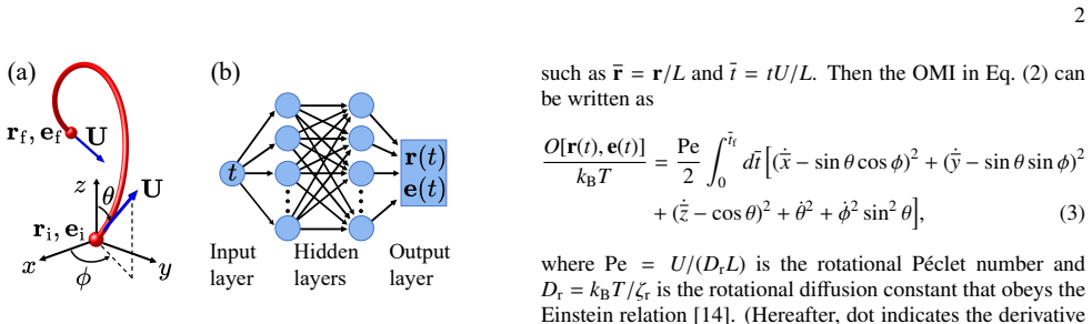
The central object is the Onsager-Machlup integral (OMI), the time integral of the Rayleighian measured relative to its deterministic minimum. For the 3D ABP it takes the dimensionless form O ∝ ∫[(ẋ−sinθ cosφ)² + (ẏ−sinθ sinφ)² + (ż−cosθ)² + θ̇² + φ̇² sin²θ] dt, with the Péclet number as prefactor. The Rayleighian is constructed by adding the active power ζ_t U·v to the dissipation function, so the Onsager-Machlup principle applies even though the active force has no free energy. The minimization is carried out by fully connected neural networks that parameterize r(t) and e(t), with time derivatives computed by automatic differentiation and boundary conditions enforced as soft constraints

What would settle it

Compute the Euler-Lagrange residuals of the optimized helical paths; if the residuals do not vanish along the trajectory, or if retraining from many random initializations converges to different OMI values, then the reported H-path is not the true most probable path.

Watch

Extended reading notes

Core claim

For a 3D active Brownian particle with prescribed initial and final positions and orientations, the most probable path is obtained by minimizing the dimensionless Onsager-Machlup integral. Direct neural-network minimization reveals that, as the final time increases (or as the apparent velocity x_f/t_f decreases), the most probable path transitions from a straight in-plane I-path, to a curved planar U-path, to a three-dimensional helical H-path that uses the extra transverse dimension to lower the OMI. When the final orientation includes an extra 2π rotation, a competing in-plane ℓ-path appears. The I- and U-path results match the known 2D analytical solutions, while the H-paths are new; the

Load-bearing premise

The central assumption is that the trained neural networks reach the global minimum of the Onsager-Machlup integral for the helical paths; the paper provides no independent check that these paths are true global minima rather than local-minimum artifacts.

Editorial extensions

If this is right

The I→U→H transition implies that apparent velocity x_f/t_f and final time are control parameters for path geometry, allowing phase diagrams for most probable paths in active matter.
The 2D agreement for I- and U-paths shows the neural minimization reproduces known analytical results, so the method can serve as a benchmark for other variational approaches.
Boundary orientations can shift transition lines substantially, meaning experimental preparation of initial and final orientations can select between planar and helical transition paths.
The same active Rayleighian construction with added active power can be applied to other nonequilibrium and nonreciprocal active systems to compute their most probable transition paths.
The OMI and entropy change evaluated along the most probable path provide direct estimates of the dissipation and time-reversal asymmetry of the dominant transition route.

Reading between the lines

Editorial extensions of the paper, not claims the author makes directly.

Although the paper focuses on a free particle, the same neural variational framework should extend to ABPs in external potentials or with obstacles, where rare transitions between metastable states become physically relevant.
The reported discontinuity in curvature and torsion at the I→U and U→H transitions hints at a buckling-like bifurcation; if pursued, an analogy with elastica theory might yield analytic estimates for the transition lines.
If helical most probable paths are genuinely the global minima, they should be observable in tracking experiments of self-propelled colloids or microswimmers with prescribed start and end configurations, where the curvature and torsion signatures could be measured directly.
The method could be pushed further by maximizing the modified, shifted OMI rather than minimizing it, giving access to cumulant generating functions and fluctuation statistics beyond the single most probable path.

Share X Bluesky LinkedIn Reddit HN

Signed reviews

No signed human review yet.

Editorial analysis

A structured set of objections, weighed in public.

Desk editor's note, referee report, and a circularity audit.

Desk Editor's Note

read the letter

Quick take on arXiv:2511.16178. The paper does a straightforward, honest thing: it takes the Onsager-Machlup integral for a 3D active Brownian particle, builds it from the Rayleighian with active power, and minimizes it with neural networks. The genuinely new piece is that in 3D you get a helical H-path branch plus boundary-condition-dependent phase diagrams for theta_f=pi/2 and 5pi/2. That is a real extension beyond the 2D analysis in Ref. [6], and the I- and U-path results match the 2D analytical line, which is the right validation.

The conceptual part is solid. The OMI derivation in Eqs. (1)-(3) is clean; Pe multiplies the whole functional and cancels out of the argmin, so there is no circular fitting. The curvature/torsion order parameters are a sensible way to classify the branches. The observation that changing theta_f by 2pi changes the transition structure is a good one.

The soft spot is exactly where the reader points: the H-path branch and the phase boundaries that involve it rest entirely on the NN minimization. The authors note themselves that the Euler-Lagrange equations are only necessary, not sufficient, for a minimum. They do not show an Euler-Lagrange residual, a second variation, seed-to-seed variance, or a comparison with a shooting method for the EL equations. Without that, the claim that the out-of-plane degrees of freedom 'permit trajectories with a lower OMI' is plausible but not demonstrated to be the global minimum. I would not call it a fatal flaw, because the 2D validation gives real confidence in the optimizer, and the I/U branches line up. But the H-region phase boundaries in Figs. 2(f) and 3(f) are not yet fully supported.

A smaller point: the active Rayleighian from Ref. [23] is stated rather than defended. That is fine for a Letter, but it should be explicit that the entire path-probability functional depends on that modeling choice. The classification thresholds for curvature/torsion are also not pinned down; minor.

If I were the editor: send it to peer review. The result is useful to people who compute transition paths in active matter, and the missing convergence evidence is checkable in a revision. I would want the authors to add one independent check for the helical branch, and report seed variance, before I believed the phase diagram completely. It is worth a serious referee's time.

Referee Report

3 major / 4 minor

Summary. The paper proposes a neural-network method to determine the most probable path (MPP) of a three-dimensional active Brownian particle (ABP) by directly minimizing the Onsager-Machlup integral (OMI). The OMI is constructed from a Rayleighian that includes the active power of the self-propulsion (Eqs. (1)-(3)), and the minimization is performed with fully connected neural networks parameterizing the position and orientation as functions of time (Eq. (6)). For boundary conditions with θ_f = π/2, the reported MPPs change from straight in-plane paths (I) to curved in-plane paths (U) and then to three-dimensional helical paths (H) as the final time increases (Fig. 2). For θ_f = 5π/2, the paper reports H-paths and a later in-plane ℓ-path (Fig. 3). The OMI values for the I- and U-paths agree with the 2D analytical results of Ref. [6], while the H-paths are new. The paper claims that the phase diagrams in Figs. 2(f) and 3(f) describe the true most probable paths of the 3D ABP.

Significance. If the central claim is correct, the work provides a general numerical route to transition paths in higher-dimensional active systems without solving nonlinear Euler-Lagrange equations. The derivation of the OMI from the Rayleighian is algebraically clean and the cancellation of the Péclet number from the argmin is a useful simplification. The validation against the 2D analytical results for the I- and U-paths is a genuine strength. The discovery of helical most probable paths, if confirmed to be global minima, would be an interesting and nontrivial result with potential implications for optimal transport and rare-event dynamics in active matter. However, the H-path regime currently rests entirely on the neural-network optimization, and the absence of an independent check of global minimality leaves the central phase diagram claim insufficiently supported.

major comments (3)

[Minimization of OMI by NN; Figs. 2(e), 2(f), 3(e), 3(f)] The phase diagrams for the H-paths are supported only by the NN minimization. The I- and U-paths are cross-validated against the analytical 2D results of Ref. [6], but no independent check is provided for the H-path regime. The paper itself notes that the Euler-Lagrange equations are only necessary conditions (text after Eq. (3)) and that convergence to a minimum is not guaranteed. The OMI is non-convex in the joint position-orientation space, so Adam may settle at a local minimum. Please provide at least one of the following for representative H-path parameters: (i) an Euler-Lagrange residual check, (ii) a second-variation (Jacobi) test, (iii) a seed-to-seed variance analysis, or (iv) a comparison with a different optimizer or a boundary-value solver. Without such a check, the claim that the H-paths are the MPPs, and hence the phase boundaries in Figs. 2(f) and 3(f), is not established.
[Figs. 2(d) and 3(d)] The classification into I-, U-, and H-paths (and ℓ-paths) is described qualitatively: 'For tf ≳9' and 'For tf ≳12' in Fig. 2(d), and 'the torsion decreases to zero' / 'a small annulus appears' in Fig. 3. No quantitative thresholds for average curvature and torsion are stated, nor is the definition of 'H-path' (e.g., a threshold on the circular projection or on torsion) given. Since the phase diagrams in Figs. 2(f) and 3(f) are built on this classification, the criteria must be specified precisely, otherwise the boundaries are not reproducible.
[Minimization of OMI by NN] The training setup is under-specified. The paper states Adam is used and gives the network architecture and boundary-penalty weights, but it does not report the learning rate, number of training epochs, loss values at convergence, or the number of independent initializations. This is important because the OMI minimization is non-convex and the reported H-paths may depend on the random initialization of the networks. Please provide these details and, if multiple runs were performed, report the variance of the OMI and of the path geometry.

minor comments (4)

[Eq. (6) and Fig. 1(b)] The text says the NNs output 'position r(t) and orientation e(t)', and Eq. (6) uses K = r, e. However, the boundary conditions are given in terms of angles θ and φ, and the network count is described as 'five NNs'. Please clarify whether the orientation network outputs the Cartesian unit vector e or the angles (θ, φ). If e is output directly, a unit-norm constraint must be imposed; if angles are output, the notation K = e is confusing.
[Eq. (3) and Eq. (6)] The same symbol O is used for the dimensional OMI in Eq. (3), for the dimensionless OMI O = 2O/(k_B T Pe), and for the loss term in Eq. (6). Similarly S is used both for the entropy change in Eq. (5) and for its dimensionless version. Please use distinct symbols (e.g., O, Õ, and J_loss) to avoid ambiguity.
[Figs. 2(f) and 3(f)] The black dashed line in Fig. 2(f) and the transition line in Fig. 3(f) are described as 'a guide for the eye'. It would be useful to state how these guides were drawn and to show error bars or confidence regions if the phase boundaries are estimated from noisy OMI comparisons.
[General] The paper does not mention the Péclet number value used in the simulations. Since Pe cancels in the minimization, the MPP is independent of Pe, but the validity of the OMI as the path action may require Pe sufficiently large to neglect possible boundary/determinant terms in the discretized path integral. A brief comment on this would be helpful.

Circularity Check

0 steps flagged · score 0.0 of 10

No significant circularity: the OMI is derived from the Rayleighian, the NN minimization is direct, and self-citations are not load-bearing.

full rationale

The paper's claimed derivation is self-contained at the level of its own equations. The OMI in Eq. (3) follows algebraically from the Rayleighian R = Φ − Ẇ_a: minimizing R with respect to v and ω gives v = U and ω = 0, and R − R_min reduces exactly to (ζ_t/2)(v−U)^2 + (ζ_r/2)ω^2, so Eq. (2) is not an independently fitted input. The active-power term Ẇ_a = ζ_t U·v is a standard modeling assumption cited to Ref. [23], but the derivation of the path weight from the resulting Langevin dynamics is explicit and not equivalent to assuming the 3D helical answer. The NN loss J in Eq. (6) contains only the OMI plus boundary penalty terms; Pe multiplies the whole action and cancels from the argmin, and no parameter is fitted to the I/U/H classifications. The 2D analytical line from Ref. [6] is used only as a validation benchmark for the I/U branches, not as an input that forces the H-path phase diagrams; the H-paths in Figs. 2(f) and 3(f) are numerical outputs of the minimization. Self-citations to Refs. [6,23,32] are present, but they supply the published model and method components, and the central 3D transition result is not derived from them. The manuscript's own caveat that the Euler-Lagrange equations are only necessary and that NN solutions may be local minima is a correctness/verification limitation, not a circularity: an unverified global minimum is an evidence gap, not equation-level equivalence. Thus no step reduces a claimed prediction to its own input.

Assumptions & free parameters 1 free parameters · 4 assumptions · 0 invented entities

The central claim carries no fitted physical parameters; Pe is an overall prefactor that does not affect the minimizer. The main assumptions are the active Rayleighian from prior literature and the validity of the Onsager-Machlup path weight, plus the numerical assumption that NN solutions are global minima.

free parameters (1)

Boundary penalty weights w_i, w_f = 100
Chosen by hand in the loss (Eq. 6) to enforce Dirichlet conditions; no sensitivity analysis reported. Not a physical parameter but a numerical hyperparameter affecting whether converged solutions satisfy BCs.

assumptions (4)

domain assumption Active Rayleighian R = Phi - W_a with W_a = zeta_t U . v
Eqs. (1)-(2) depend on this extension of Onsager's principle to active systems, adopted from Ref. [23]; not derived here.
domain assumption Conditional path probability is P = C exp(-O/(2 k_B T))
Standard Onsager-Machlup weight for Gaussian fluctuations, applied here to an ABP; assumed valid for active dynamics and used to define the MPP as the OMI minimizer.
standard math omega is perpendicular to e, so omega^2 = theta_dot^2 + phi_dot^2 sin^2(theta)
Standard spherical parametrization of a unit vector; stated before Eq. (3) and used throughout.
domain assumption Local detailed balance gives the bath entropy change in Eqs. (4)-(5)
Used to compute entropy change along the MPP; cited to [38,39] but not derived in this paper.

how reviews work

0 comments

Cite this review

Pith. "Pith review of Neural optimization of the most probable paths of 3D active Brownian particles." pith.science (2026). https://pith.science/paper/FCTNIHZI

@misc{pith2026251116178,
  author       = {Pith},
  title        = {Pith review of: Neural optimization of the most probable paths of 3D active Brownian particles},
  year         = {2026},
  howpublished = {\url{https://pith.science/paper/FCTNIHZI}},
  note         = {Machine review of arXiv:2511.16178}
}

read the original abstract

We develop a variational neural-network framework to determine the most probable path (MPP) of a 3D active Brownian particle (ABP) by directly minimizing the Onsager-Machlup integral (OMI). To obtain the OMI, we use the Onsager-Machlup variational principle for active systems and construct the Rayleighian of the ABP by including its active power. This approach reveals geometric transitions of the MPP from in-plane I- and U-shaped paths to 3D helical paths as the final time and net displacement are varied. We also demonstrate that the initial and final boundary conditions have a significant impact on the MPPs. Our results show that neural optimization combined with the Onsager-Machlup variational principle provides an efficient and versatile framework for exploring optimal transition pathways in active and nonequilibrium systems.

Figures

Figures reproduced from arXiv: 2511.16178 by the authors.

**Figure 2.** FIG. 2. NN solutions of the MPP of a 3D ABP for di [PITH_FULL_IMAGE:figures/full_fig_p003_2.png] view at source ↗

**Figure 3.** FIG. 3. NN solutions of the MPP of a 3D ABP for di [PITH_FULL_IMAGE:figures/full_fig_p004_3.png] view at source ↗

Discussion (0). Continue with ORCID to comment.

Forward citations

Cited by 1 Pith paper

Reviewed papers in the Pith corpus that reference this work. Sorted by Pith novelty score. Full citation record

Covariant Onsager and Onsager-Machlup principles for active and inertial dynamics
cond-mat.soft 2026-04 unverdicted novelty 7.0 of 10

Covariant Onsager and Onsager-Machlup principles are derived for active matter with inertia, yielding geometrically consistent dynamics and path probabilities that satisfy the detailed fluctuation theorem.

Reference graph

Works this paper leans on

51 extracted references · 1 linked inside Pith · cited by 1 Pith paper

[6]

Yasuda, and K

K. Yasuda, and K. Ishimoto, Most probable path of an active Brownian particle, Phys. Rev. E 106, 064120 (2022)

2022
[23]

H. Wang, T. Qian, and X. Xu, Onsager’s variational principle in active soft matter, Soft Matter 17, 3634 (2021)

2021
[1]

Lauga,The Fluid Dynamics of Cell Motility(Cambridge Uni- versity Press, Cambridge, 2020)

E. Lauga,The Fluid Dynamics of Cell Motility(Cambridge Uni- versity Press, Cambridge, 2020)

2020
[2]

Gompper, R

G. Gompper, R. G. Winkler, T. Speck, A. Solon, C. Nardini, F. Peruani, H. L¨owen, R. Golestanian, U. B. Kaupp, L. Alvarezet al., The 2020 motile active matter roadmap, J. Phys.: Condens. Matter 32, 193001 (2020)

2020
[3]

Romanczuk, M

P. Romanczuk, M. B ¨ar, W. Ebeling, B. Lindner, and L. Schimansky-Geier, Active Brownian particles, Eur. Phys. J.: 6 Spec. Top. 202, 1 (2012)

2012
[4]

Fily and M

Y . Fily and M. C. Marchetti, Athermal Phase Separation of Self- Propelled Particles with No Alignment, Phys. Rev. Lett. 108, 235702 (2012)

2012
[5]

M. E. Cates and J. Tailleur, Motility-Induced Phase Separation, Annu. Rev. Condens. Matter Phys. 6, 219 (2015)

2015
[7]

A. Das, B. Kuznets-Speck, and D. T. Limmer, Direct Evalu- ation of Rare Events in Active Matter from Variational Path Sampling, Phys. Rev. Lett. 128, 028005 (2022)

2022

Show all 51 references

[8]

Crisanti and M

A. Crisanti and M. Paoluzzi, Most probable path of ac- tive Ornstein-Uhlenbeck particles, Phys. Rev. E 107, 034110 (2023)

2023
[9]

Dutta, Most probable paths for active Ornstein-Uhlenbeck particles, Phys

S. Dutta, Most probable paths for active Ornstein-Uhlenbeck particles, Phys. Rev. E 107, 054130 (2023)

2023
[10]

Onsager and S

L. Onsager and S. Machlup, Fluctuations and irreversible pro- cesses, Phys. Rev. 91, 1505 (1953)

1953
[11]

Machlup and L

S. Machlup and L. Onsager, Fluctuations and Irreversible Pro- cess. II. Systems with Kinetic Energy, Phys. Rev. 91, 1512 (1953)

1953
[12]

M. Doi, J. Zhou, Y . Di and X. Xu, Application of the Onsager- Machlup integral in solving dynamic equations in nonequilib- rium systems, Phys. Rev. E 99, 063303 (2019)

2019
[13]

Doi, Onsager’s variational principle in soft matter, J

M. Doi, Onsager’s variational principle in soft matter, J. Phys.: Condens. Matter 23, 284118 (2011)

2011
[14]

Doi,Soft Matter Physics(Oxford University Press, Oxford, England, 2013)

M. Doi,Soft Matter Physics(Oxford University Press, Oxford, England, 2013)

2013
[15]

Onsager, Reciprocal relations in irreversible processes

L. Onsager, Reciprocal relations in irreversible processes. I, Phys. Rev. 37, 405 (1931)

1931
[16]

Onsager, Reciprocal relations in irreversible processes

L. Onsager, Reciprocal relations in irreversible processes. II, Phys. Rev. 38, 2265 (1931)

1931
[17]

X. Xu, U. Thiele, and T. Qian, A Variational approach to thin film hydrodynamics of binary mixtures, J. Phys.: Condens. Matter 27, 085005 (2015)

2015
[18]

Okamoto, Y

R. Okamoto, Y . Kanemori, S. Komura, and J.-B. Fournier, Re- laxation dynamics of two-component fluid bilayer membranes, Eur. Phys. J. E 39, 52 (2016)

2016
[19]

Man and M

X. Man and M. Doi, Vapor-induced motion of liquid droplets on an inert substrate, Phys. Rev. Lett. 119, 044502 (2017)

2017
[20]

Zhou and M

J. Zhou and M. Doi, Dynamics of viscoelastic filaments based on Onsager principle, Phys. Rev. Fluids 3, 084004 (2018)

2018
[21]

Doi, Onsager principle in polymer dynamics, Prog

M. Doi, Onsager principle in polymer dynamics, Prog. Polym. Sci. 112, 101339 (2021)

2021
[22]

Zhang, M

Y .-H. Zhang, M. Deserno, and Z.-C. Tu, Dynamics of active nematic defects on the surface of a sphere, Phys. Rev. E 102, 012607 (2020)

2020
[24]

Ackermann and M

J. Ackermann and M. B. Amar, Onsager’s variational principle in proliferating biological tissues, in the presence of activity and anisotropy, Eur. Phys. J. Plus 138, 1103 (2023)

2023
[25]

Taniguchi and E

T. Taniguchi and E. G. D. Cohen, Onsager-Machlup Theory for Nonequilibrium Steady States and Fluctuation Theorems, J. Stat. Phys. 126, 1 (2007)

2007
[26]

Taniguchi and E

T. Taniguchi and E. G. D. Cohen, Inertial Effects in Nonequi- librium Work Fluctuations by a Path Integral Approach, J. Stat. Phys. 130, 1 (2008)

2008
[27]

G. E. Karniadakis, I. G. Kevrekidis, L. Lu, P. Perdikaris, S. Wang, and L. Yang, Physics-informed machine learning, Nat. Rev. Phys. 3, 422 (2021)

2021
[28]

Rohanizadegan, H

Y . Rohanizadegan, H. Li, and J. Z. Y . Chen, Neural-network- based solver for vesicle shapes predicted by the Helfrich model, Soft Matter 20, 5359 (2024)

2024
[29]

A. R. Dulaney and J. F. Brady, Machine learning for phase be- havior in active matter systems, Soft Matter 17, 6808 (2021)

2021
[30]

Colen, M

J. Colen, M. Han, R. Zhang, S. A. Redford, L. M. Lemma, L. Morgan, P. V . Ruijgrok, R. Adkins, Z. Bryant, Z. Dogic, M. L. Gardel, J. J. de Pablo, and V . Vitelli, Machine learning active-nematic hydrodynamics, Proc. Natl. Acad. Sci. U.S.A. 118, e2016708118 (2021)

2021
[31]

H. Wang, B. Zou, J. Su, D. Wang, and X. Xu, Variational meth- ods and deep Ritz method for active elastic solids, Soft Matter 18, 6015 (2022)

2022
[32]

Z. Li, B. Zou, H. Wang, J. Su, D. Wang, and X. Xu, Deep Learning-Based Computational Method for Soft Matter Dy- namics: Deep Onsager-Machlup Method, Commun. Comput. Phys. 37, 353 (2025)

2025
[33]

Rumelhart, G

D. Rumelhart, G. Hinton, and R. Williams, Learning represen- tations by back-propagating errors, Nature 323, 533 (1986)

1986
[34]

W. Wei, T. Gao, X. Chen, and J. Duan, An optimal control method to compute the most likely transition path for stochastic dynamical systems with jumps, Chaos 32, 051102 (2022)

2022
[35]

L. S. Lin, K. Yasuda, K. Ishimoto, and S. Komura, Emergence of odd elasticity in a microswimmer using deep reinforcement learning, Phys. Rev. Res. 6, 033016 (2024)

2024
[36]

Orland, Generating transition paths by Langevin bridges, J

H. Orland, Generating transition paths by Langevin bridges, J. Chem. Phys. 134, 174114 (2011)

2011
[37]

(3): d dt (˙x−sinθcosϕ)=0, d dt (˙y−sinθsinϕ)=0, d dt (˙z−cosθ)=0, ˙xcosθcosϕ+ ˙ycosθsinϕ− ˙zsinθ− ˙ϕ2 sinθcosθ+ ¨θ=0, ˙xsinϕ− ˙ycosϕ−2 ˙θ ˙ϕcosθ− ¨ϕsinθ=0

The following equations are the Euler-Lagrange equations that minimize the OMI in Eq. (3): d dt (˙x−sinθcosϕ)=0, d dt (˙y−sinθsinϕ)=0, d dt (˙z−cosθ)=0, ˙xcosθcosϕ+ ˙ycosθsinϕ− ˙zsinθ− ˙ϕ2 sinθcosθ+ ¨θ=0, ˙xsinϕ− ˙ycosϕ−2 ˙θ ˙ϕcosθ− ¨ϕsinθ=0
[38]

Sekimoto,Stochastic Energetics(Springer, Berlin/Heidelberg, 2010)

K. Sekimoto,Stochastic Energetics(Springer, Berlin/Heidelberg, 2010)

2010
[39]

Seifert, Stochastic thermodynamics, fluctuation theorems and molecular machines, Rep

U. Seifert, Stochastic thermodynamics, fluctuation theorems and molecular machines, Rep. Prog. Phys. 75, 126001 (2012)

2012
[40]

Audoly and Y

B. Audoly and Y . Pomeau,Elasticity and Geometry: From hair curls to the nonlinear response of shells(Oxford Univ. Press, Oxford, 2010)

2010
[41]

Fruchart, R

M. Fruchart, R. Hanai, P. B. Littlewood, and V . Vitelli, Non- reciprocal phase transitions, Nature 592, 363 (2021)

2021
[42]

Fruchart, C

M. Fruchart, C. Scheibner, and V . Vitelli, Odd Viscosity and Odd Elasticity, Annu. Rev. Condens. Matter Phys. 14, 471 (2023)

2023
[43]

Z. You, A. Baskaran, and M. C. Marchetti, Nonreciprocity as a generic route to traveling states, Proc. Nat. Acad. Sci. 117, 19767 (2020)

2020
[44]

S. Saha, J. Agudo-Canalejo, and R. Golestanian, Scalar Active Mixtures: The Nonreciprocal Cahn-Hilliard Model, Phys. Rev. X 10, 041009 (2020)

2020
[45]

M. Liu, Z. Hou, H. Kitahata, L. He, and S. Komura, Non- reciprocal phase separations with non-conserved order parame- ters, J. Phys. Soc. Jpn. 92, 093001 (2023)

2023
[46]

Tateyama, H

Y . Tateyama, H. Ito, S. Komura, and H. Kitahata, Pattern dy- namics of the non-reciprocal Swift-Hohenberg model, Phys. Rev. E 110, 054209 (2024)

2024
[47]

Yasuda, A

K. Yasuda, A. Kobayashi, L.-S. Lin, Y . Hosaka, I. Sou, and S. Komura, The Onsager-Machlup integral for non-reciprocal sys- tems with odd elasticity, J. Phys. Soc. Jpn. 91, 015001 (2022)

2022
[48]

Yasuda, K

K. Yasuda, K. Ishimoto, A. Kobayashi, L.-S. Lin, I. Sou, Y . Hosaka, and S. Komura, Time-correlation functions for odd Langevin systems, J. Chem. Phys. 157, 095101 (2022)

2022
[49]

Yasuda, Irreversibility of stochastic state transitions in Langevin systems with odd elasticity, Phys

K. Yasuda, Irreversibility of stochastic state transitions in Langevin systems with odd elasticity, Phys. Rev. E 109, 064116 (2024). 7

2024
[50]

Yasuda, K

K. Yasuda, K. Ishimoto, and S. Komura, Statistical formulation of the Onsager-Machlup variational principle, Phys. Rev. E 110, 044104 (2024)

2024
[51]

Yasuda, K

K. Yasuda, K. Ishimoto, and S. Komura, Demon’s variational principle for informational active matter, arXiv:2510.13145

arXiv

Pith tools

Reviewed August 3, 2026 · model on record in the stance chip above.

[1] [6]

Yasuda, and K

K. Yasuda, and K. Ishimoto, Most probable path of an active Brownian particle, Phys. Rev. E 106, 064120 (2022)

2022

[2] [23]

H. Wang, T. Qian, and X. Xu, Onsager’s variational principle in active soft matter, Soft Matter 17, 3634 (2021)

2021

[3] [1]

Lauga,The Fluid Dynamics of Cell Motility(Cambridge Uni- versity Press, Cambridge, 2020)

E. Lauga,The Fluid Dynamics of Cell Motility(Cambridge Uni- versity Press, Cambridge, 2020)

2020

[4] [2]

Gompper, R

G. Gompper, R. G. Winkler, T. Speck, A. Solon, C. Nardini, F. Peruani, H. L¨owen, R. Golestanian, U. B. Kaupp, L. Alvarezet al., The 2020 motile active matter roadmap, J. Phys.: Condens. Matter 32, 193001 (2020)

2020

[5] [3]

Romanczuk, M

P. Romanczuk, M. B ¨ar, W. Ebeling, B. Lindner, and L. Schimansky-Geier, Active Brownian particles, Eur. Phys. J.: 6 Spec. Top. 202, 1 (2012)

2012

[6] [4]

Fily and M

Y . Fily and M. C. Marchetti, Athermal Phase Separation of Self- Propelled Particles with No Alignment, Phys. Rev. Lett. 108, 235702 (2012)

2012

[7] [5]

M. E. Cates and J. Tailleur, Motility-Induced Phase Separation, Annu. Rev. Condens. Matter Phys. 6, 219 (2015)

2015

[8] [7]

A. Das, B. Kuznets-Speck, and D. T. Limmer, Direct Evalu- ation of Rare Events in Active Matter from Variational Path Sampling, Phys. Rev. Lett. 128, 028005 (2022)

2022