REVIEW 3 major objections 5 minor 65 references
MAGNETS claims that an inherently interpretable architecture can match strong black-box models on time series regression by learning binary masks over time and channels, summing the selected values into a few concepts, and predicting linear
Reviewed by Pith at T0; open to challenge. T0 means a machine referee read the full paper against a public rubric. the ladder, T0–T4 →
T0 review · deepseek-v4-flash
2026-08-03 18:44 UTC pith:IYUGC2WS
load-bearing objection MAGNETS is a genuinely useful interpretable TSER architecture, but the 'closely matches black-box' claim needs scoping to sum-representable targets; the Benzene gap is the tell. the 3 major comments →
When, How Long and How Much? Interpretable Neural Networks for Time Series Regression by Learning to Mask and Aggregate
The pith
A machine-rendered reading of the paper's core claim, the machinery that carries it, and where it could break.
Core claim
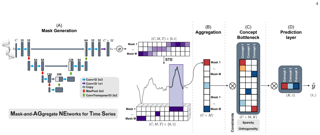
On its own terms, the paper's discovery is that annotation-free concept discovery for time series regression is achievable through a mask-and-aggregate design. For each input, a 1D U-Net emits M binary masks per channel; each mask is applied to the raw signal and the surviving values are summed, so a feature encodes both when the region occurs and how large the signal is there. A linear concept bottleneck combines these channel-mask features into K concepts under L1 sparsity and orthogonality, and the prediction is a linear combination of concepts. On four synthetic datasets the learned masks reconstruct the true temporal logic (area above a threshold, conditional areas defined by channel co
What carries the argument
The central mechanism is the binary mask plus summation. A per-input 1D U-Net emits logits that are binarized with a straight-through Gumbel-softmax estimator, yielding masks in {0,1} per channel, mask index, and time step; each channel-mask pair yields z equal to the sum over time of the masked raw values, a scalar that merges duration and intensity. A linear bottleneck with L1 sparsity and orthogonality regularization turns these sums into a compact set of concepts, and a linear head maps concept activations to the prediction. The load-bearing idea is that masks do the localization, sums do the quantification, and the linear bottleneck does feature interaction — so the whole decision path
Load-bearing premise
The load-bearing premise is that the target is well approximated by a linear combination of sums of raw input values over selected intervals; if the target genuinely depends on variance, slope, frequency content, or products of channels at the same time, the architecture cannot express it regardless of how good the masks are.
What would settle it
Generate a synthetic time series regression dataset whose target is the variance, or the slope, of a flagged region rather than its sum. If MAGNETS's error stays substantially above a simple model that explicitly computes that statistic, the summation bottleneck is the cause. A second check: a target defined by the product of two channels' values at the same time step, which the linear bottleneck also cannot express.
If this is right
- If the claim holds, domain users can trace any prediction to concrete intervals on concrete sensors, because the only quantities that affect the output are sums of raw values over binary masks.
- Concept bottlenecks no longer require concept labels: the model discovers concepts from raw data, removing the main obstacle to concept-based interpretability in time series.
- Multivariate interactions are representable despite an additive-looking pipeline, because masks are per-channel and the bottleneck linearly combines channels; this is what enables it to beat pure additive baselines on conditional-area tasks.
- On the evaluated benchmarks, accuracy can stay close to a flexible CNN, so transparency is not bought at the cost of a large accuracy gap.
Where Pith is reading between the lines
- My inference: the summation aggregation is the real boundary of the method; replacing it with a small set of interpretable alternates (peak value, variance, slope, or count of threshold crossings) while keeping the mask and linear-bottleneck skeleton would likely extend the same transparency to targets that depend on signal shape rather than area.
- My inference: because masks are input-dependent and the bottleneck is linear, the trained model can double as a hypothesis generator for domain experts — patterns it isolates on real data (for example, bridge displacement when train load exceeds a threshold) can be checked as candidate physical rules.
- My inference: the same architecture should transfer to time series classification with minimal change, since the mask-and-aggregate concepts are class-agnostic; a linear softmax head would preserve the explanation pathway.
Editorial analysis
A structured set of objections, weighed in public.
Referee Report
Summary. The paper proposes MAGNETS, an inherently interpretable neural architecture for time series extrinsic regression (TSER). A mask-generation network (1D U-Net) produces input-dependent binary masks per channel; masked raw input values are aggregated by summation into scalar features, mapped linearly to a small set of concepts with sparsity and orthogonality regularization, and finally combined linearly into the prediction. The authors evaluate on four synthetic datasets with known ground-truth temporal rules and four real-world TSER benchmarks, reporting that MAGNETS closely approaches black-box CNN accuracy while outperforming interpretable baselines, and that its masks are more faithful to ground-truth regions than post-hoc Integrated Gradients and DeepLIFT attributions. Code and datasets are publicly available.
Significance. If the central claim held, MAGNETS would be a useful contribution: it offers an annotation-free, temporally localized concept-bottleneck architecture for TSER, with a transparent additive decomposition from masked inputs to the final prediction. The paper's strengths include public code, synthetic benchmarks with ground-truth temporal logic, quantitative explanation-quality comparisons against post-hoc methods, and a clear architectural story. However, the architecture's expressiveness is restricted to linear combinations of sums of raw input values over binary-selected temporal regions; the synthetic targets are generated from exactly this class. Consequently, the paper's general claim that MAGNETS 'closely matches' black-box accuracy is only supported for sum-representable targets, and the real-world results show a large accuracy gap on BenzeneConcentration. The paper needs scope revision and additional experiments before the claims are sustainable.
major comments (3)
- [§III-B–D, §VI, Table III] The expressiveness limitation is load-bearing and undermines the general claim. Equations (8), (10), and (13) make the final predictor exactly w0 + Σ_k w_k (b_k + Σ_{c,m} β_{c,m,k} Σ_t x_{c,t} m_{c,m,t}). This class cannot represent targets that depend on variance, slope, frequency, or nonlinear cross-channel products at the same time step, regardless of mask quality. The synthetic datasets in §IV-B are all conditional areas, i.e., precisely this sum class, so success there is expected. On real data, Table III shows the largest gap exactly on BenzeneConcentration (MAGNETS RMSE 1.2008 vs CNN 0.3994, about 3× worse), consistent with a target outside the expressible class. The conclusion acknowledges 'the current aggregation mechanism is limited to summation,' but the abstract and introduction present MAGNETS as a general interpretable TSER solution. The authors should either restrict the c
- [§IV-D, Tables II–III] All reported accuracy results are point estimates from a single run with no repeated seeds, confidence intervals, or significance tests. Some central comparisons are close: on WindTurbinePower MAGNETS is 23.65 vs CNN 23.41, and on HouseholdPowerC1 Lasso is 151.99 vs MAGNETS 153.20. Without repeated-run statistics or paired testing, the claim of 'closely matches black-box accuracy' and the ranking against interpretable baselines are not statistically supported. This is fixable and important for the paper's main empirical claim.
- [§IV-B, Table II] The synthetic evaluation is aligned with the model's inductive bias: every synthetic target is defined as an area under a curve over a binary-selected region, which is precisely the class MAGNETS can represent. The strong results in Table II therefore do not demonstrate general TSER capability. To make the interpretability and accuracy claims convincing, the authors should add synthetic datasets whose targets require non-sum statistics (e.g., variance, slope, or cross-channel products) and report the resulting accuracy and whether the masks still recover the relevant regions. This would either substantiate the general claim or clarify the intended scope.
minor comments (5)
- [§V-C, Tables II–III] The tables label Optimal Summaries as '[21]' but the text cites it as [53]. Please correct the reference tags.
- [§V-C, Tables II–III] The regularization weight is called λ_ortho in the text (Eqs. 12 and 14) but λ_cos in the tables. Please unify the notation.
- [Throughout] There are several typos: 'to to' in the introduction, 'bottlneck' in §III-C, 'disciminative' in §II-B, 'Dimicorresponds' in the Fig. 4 caption, 'times teps' in §V-B, 'predictions predictions' in §II-B, and 'a explicit weight' in §III-D. A copyedit pass is needed.
- [§V-B, Figures 3–4] The heatmap color scales in Fig. 3 and Fig. 4 are not described; it is difficult to tell whether the colorbar ranges are comparable across panels. Please add explicit colorbar labels and normalization details.
- [§IV-D] The CNN baseline is described as matched in capacity to the masking network, but no architectural details (number of layers, kernel sizes, pooling) are given. Please provide enough detail for reproducibility.
Circularity Check
No significant circularity; MAGNETS' masks-to-concepts-to-output pathway is the model definition, and benchmarks are external/independent.
full rationale
The paper's core derivation is an architectural construction, not a fitted quantity presented as a prediction. The prediction is defined as a linear combination of concepts, each a linear combination of masked sums (Eqs. 6-13); the masks are learned from the input. Nothing in this chain is fit to a target and then renamed as an independent discovery. The synthetic benchmarks are generated from rules of the same general form (areas under selected regions), but this is an expressiveness match, not a circularity: the experiments test whether gradient-based learning can recover the known masks, and the CNN baseline often fails to do so despite being in the same broad function class. Real-world results are measured against external TSER archive data, and the paper explicitly acknowledges the summation-only limitation. Self-citations [16] and [60] supply related work and a dataset, but they are not load-bearing for the architecture or the empirical claims; no uniqueness theorem or prior result by the authors is invoked to force the method. The main caveat is scoping: the 'closely matches black-box accuracy' claim is weaker for BenzeneConcentration, and the class of representable functions is limited to sums of masked inputs. These are correctness/scope concerns, not circular derivation.
Axiom & Free-Parameter Ledger
free parameters (3)
- M (number of masks per channel) =
10
- K (number of concepts) =
3
- lambda_spars, lambda_ortho =
0 or 1
axioms (4)
- domain assumption Target functions in TSER are well approximated by linear combinations of sums over selected temporal regions.
- domain assumption The straight-through Gumbel estimator yields effective training despite binary masks.
- domain assumption Sparsity and orthogonality regularizers do not materially degrade accuracy while improving interpretability.
- domain assumption The 1D U-Net mask generator produces masks that align with human-understandable temporal semantics.
read the original abstract
Time series extrinsic regression (TSER) refers to the task of predicting a continuous target variable from an input time series. It appears in many domains, including healthcare, finance, environmental monitoring, and engineering. In these settings, accurate predictions and trustworthy reasoning are both essential. Although state-of-the-art TSER models achieve strong predictive performance, they typically operate as black boxes, making it difficult to understand which temporal patterns drive their decisions. Post-hoc interpretability techniques, such as feature attribution, aim to to explain how the model arrives at its predictions, but often produce coarse, noisy, or unstable explanations. Recently, inherently interpretable approaches based on concepts, additive decompositions, or symbolic regression, have emerged as promising alternatives. However, these approaches remain limited: they require explicit supervision on the concepts themselves, often cannot capture interactions between time-series features, lack expressiveness for complex temporal patterns, and struggle to scale to high-dimensional multivariate data. To address these limitations, we propose MAGNETS (Mask-and-AGgregate NEtwork for Time Series), an inherently interpretable neural architecture for TSER. MAGNETS learns a compact set of human-understandable concepts without requiring any annotations. Each concept corresponds to a learned, mask-based aggregation over selected input features, explicitly revealing both which features drive predictions and when they matter in the sequence. Predictions are formed as combinations of these learned concepts through a transparent, additive structure, enabling clear insight into the model's decision process. The code implementation and datasets are publicly available at https://github.com/FlorentF9/MAGNETS.
Figures


Reference graph
Works this paper leans on
-
[1]
Time series extrinsic regression,
C. W. Tan, C. Bergmeir, F. Petitjean, and G. I. Webb, “Time series extrinsic regression,”Data Mining and Knowledge Discovery, vol. 35, no. 3, pp. 1032–1060, May 2021. Available: https: //doi.org/10.1007/s10618-021-00745-9
-
[2]
Deep Learning for Time Series Classification and Extrinsic Regression: A Current Survey,
N. Mohammadi Foumani, L. Miller, C. W. Tan, G. I. Webb, G. Forestier, and M. Salehi, “Deep Learning for Time Series Classification and Extrinsic Regression: A Current Survey,”ACM Comput. Surv., vol. 56, no. 9, pp. 217:1–217:45, Apr. 2024. Available: https://dl.acm.org/doi/10.1145/3649448
doi:10.1145/3649448 2024
-
[3]
Deep learning for time series classification: a review,
H. Ismail Fawaz, G. Forestier, J. Weber, L. Idoumghar, and P.-A. Muller, “Deep learning for time series classification: a review,”Data Mining and Knowledge Discovery, vol. 33, no. 4, pp. 917–963, Jul
-
[4]
J. Chen, “Addressing spatial-temporal heterogeneity: General mixed time series analysis via latent continuity recovery and alignment,” inNeurIPS, vol. 37, pp. 17910–17946, 2024. Available: https: //doi.org/10.52202/079017-0569
-
[5]
Unsupervised feature based algorithms for time series extrinsic regression,
D. Guijo-Rubio, M. Middlehurst, G. Arcencio, D. F. Silva, and A. Bagnall, “Unsupervised feature based algorithms for time series extrinsic regression,”Data Mining and Knowledge Discovery, vol. 38, no. 4, pp. 2141–2185, Jul. 2024. Available: https: //doi.org/10.1007/s10618-024-01027-w
-
[6]
A. Dempster, F. Petitjean, and G. I. Webb, “ROCKET: Exceptionally fast and accurate time series classification using random convolutional kernels,”Data Mining and Knowledge Discovery, vol. 34, no. 5, pp. 1454–1495, Sep. 2020. Available: http://arxiv.org/abs/1910.13051
Pith/arXiv arXiv 2020
-
[7]
MultiRocket: Multiple pooling operators and transformations for fast and effective time series classification,
C. W. Tan, A. Dempster, C. Bergmeir, and G. I. Webb, “MultiRocket: Multiple pooling operators and transformations for fast and effective time series classification,”Data Mining and Knowledge Discovery, vol. 36, pp. 1623–1646, Feb. 2022. Available: http://arxiv.org/abs/2102. 00457
2022
-
[8]
Hydra: Competing convolutional kernels for fast and accurate time series classification,
A. Dempster, D. F. Schmidt, and G. I. Webb, “Hydra: Competing convolutional kernels for fast and accurate time series classification,” Data Mining and Knowledge Discovery, vol. 37, no. 5, pp. 1779–1805, May 2023. Available: https://doi.org/10.1007/s10618-023-00939-3
-
[9]
Benchmarking Deep Learning Interpretability in Time Series Predictions,
A. A. Ismail, M. Gunady, H. C. Bravo, and S. Feizi, “Benchmarking Deep Learning Interpretability in Time Series Predictions,” inNeurIPS, Vancouver, Canada, Oct. 2020. Available: http://arxiv.org/abs/2010. 13924
2020
-
[10]
TimeX++: Learning Time- Series Explanations with Information Bottleneck,
Z. Liu, T. Wang, J. Shi, X. Zheng, Z. Chen, L. Song, W. Dong, J. Obeysekera, F. Shirani, and D. Luo, “TimeX++: Learning Time- Series Explanations with Information Bottleneck,” inProceedings of the 41st International Conference on Machine Learning, 2024. Available: http://arxiv.org/abs/2405.09308
Pith/arXiv arXiv 2024
-
[11]
TIMING: Temporality-Aware Integrated Gradients for Time Series Explanation,
H. Jang, C. Kim, E. Yang, “TIMING: Temporality-Aware Integrated Gradients for Time Series Explanation,”Proceedings of the 42nd International Conference on Machine Learning, 2025. Available: https://openreview.net/forum?id=qOgKMqv9T7
2025
-
[12]
Stop explaining black box machine learning models for high stakes decisions and use interpretable models instead,
C. Rudin, “Stop explaining black box machine learning models for high stakes decisions and use interpretable models instead,”Nature Machine Intelligence, vol. 1, no. 5, pp. 206–215, May 2019. Available: https://www.nature.com/articles/s42256-019-0048-x
2019
-
[13]
Neural Additive Models: Interpretable Machine Learning with Neural Nets,
R. Agarwal, L. Melnick, N. Frosst, X. Zhang, B. Lengerich, R. Caruana, and G. Hinton, “Neural Additive Models: Interpretable Machine Learning with Neural Nets,” inNeurIPS 2021, Oct. 2021. Available: http://arxiv.org/abs/2004.13912
Pith/arXiv arXiv 2021
-
[14]
Neural additive time-series models: Explainable deep learning for multivariate time-series prediction,
W. Jo and D. Kim, “Neural additive time-series models: Explainable deep learning for multivariate time-series prediction,”Expert Systems with Applications, vol. 228, p. 120307, Oct. 2023. Available: https://linkinghub.elsevier.com/retrieve/pii/S0957417423008096
2023
-
[15]
Concept Bottleneck Models,
P. W. Koh, T. Nguyen, Y . S. Tang, S. Mussmann, E. Pierson, B. Kim, and P. Liang, “Concept Bottleneck Models,” inProceedings of the 37th International Conference on Machine Learning, 2020
2020
-
[16]
Interpretable Prognostics with Concept Bottleneck Models,
F. Forest, K. Rombach, and O. Fink, “Interpretable Prognostics with Concept Bottleneck Models,” inInformation Fusion, Dec. 2025. Available: https://doi.org/10.1016/j.inffus.2025.103427
arXiv 2025
-
[17]
Towards Automatic Concept-based Explanations,
A. Ghorbani, J. Wexler, J. Y . Zou, and B. Kim, “Towards Automatic Concept-based Explanations,” inAdvances in Neural Information Processing Systems, vol. 32, 2019. Available: https://papers.nips.cc/ paper/2019/hash/77d2afcb31f6493e350fca61764efb9a-Abstract.html
2019
-
[18]
Label- Free Concept Bottleneck Models,
T. Oikarinen, S. Das, L. M. Nguyen, and T.-W. Weng, “Label- Free Concept Bottleneck Models,” inICLR, 2023. Available: http://arxiv.org/abs/2304.06129
Pith/arXiv arXiv 2023
-
[19]
Discover-then- Name: Task-Agnostic Concept Bottlenecks via Automated Concept Discovery,
S. Rao, S. Mahajan, M. B ¨ohle, and B. Schiele, “Discover-then- Name: Task-Agnostic Concept Bottlenecks via Automated Concept Discovery,”inECCV2024. Available: http://arxiv.org/abs/2407.14499
-
[20]
Interpretable-by-Design Text Understanding with Iteratively Generated Concept Bottleneck,
J. M. Ludan, Q. Lyu, Y . Yang, L. Dugan, M. Yatskar, and C. Callison-Burch, “Interpretable-by-Design Text Understanding with Iteratively Generated Concept Bottleneck,” Apr. 2024. Available: http://arxiv.org/abs/2310.19660
Pith/arXiv arXiv 2024
-
[21]
Discovering Invariant Rationales for Graph Neural Networks
Y .-X. Wu, X. Wang, A. Zhang, X. He, and T.-S. Chua, “Discovering Invariant Rationales for Graph Neural Networks”, inICLR, 2022. Available: https://arxiv.org/abs/2201.12872
Pith/arXiv arXiv 2022
-
[22]
Interpretable extreme wind speed prediction with concept bottleneck models,
C. ˜Alvarez Rodriguez, E. Parrado-Hernandez, J. P ´erez-Aracil, L. Prieto- Godino, and S. Salcedo-Sanz, “Interpretable extreme wind speed prediction with concept bottleneck models,”Renewable Energy, vol. 231, p. 120935, Sep. 2024. Available: https://linkinghub.elsevier.com/ retrieve/pii/S0960148124010036
2024
-
[23]
A. B. Arrieta, N. Diaz-Rodriguez, J. Del Ser, A. Bennetot, S. Tabik, A. Barbado, S. Garcia, S. Gil-Lopez, D. Molina, R. Benjamins, R. Chatila, and F. Herrera, “Explainable Artificial Intelligence (XAI): Concepts, Taxonomies, Opportunities and Challenges toward Responsible AI,” inInformation Fusion, Dec. 2019. Available: http://arxiv.org/abs/1910.10045
Pith/arXiv arXiv 2019
-
[24]
Axiomatic Attribution for Deep Networks,
M. Sundararajan, A. Taly, Q. Yan, “Axiomatic Attribution for Deep Networks,”Proceedings of the 34th International Conference on Machine Learning, 2017. Available: https://proceedings.mlr.press/v70/ sundararajan17a.html
2017
-
[25]
Learning Important Features Through Propagating Activation Differences,
A. Shrikumar, P. Greenside, A. Kundaje, “Learning Important Features Through Propagating Activation Differences,” inProceedings of the 34th International Conference on Machine Learning, 2017. Available: https://proceedings.mlr.press/v70/shrikumar17a
2017
-
[26]
What went wrong and when? Instance-wise feature importance for time-series black-box models,
S. Tonekaboni, S. Joshi, K. R. Campbell, D. Duvenaud, and A. Goldenberg, “What went wrong and when? Instance-wise feature importance for time-series black-box models,” in34th Conference on Neural Information Processing Systems (NeurIPS 2020), 2020
2020
-
[27]
Explaining Time Series Predictions with Dynamic Masks,
J. Crabb ´e and M. van der Schaar, “Explaining Time Series Predictions with Dynamic Masks,” inProceedings of the 38 th International Conference on Machine Learning, vol. 139., PMLR, Jun. 2021. Available: http://arxiv.org/abs/2106.05303
Pith/arXiv arXiv 2021
-
[28]
Temporal Dependencies in Feature Importance for Time Series Predictions,
K. K. Leung, C. Rooke, J. Smith, S. Zuberi, and M. V olkovs, “Temporal Dependencies in Feature Importance for Time Series Predictions,” in ICLR2023. Available: http://arxiv.org/abs/2107.14317
-
[29]
Learning Perturbations to Explain Time Series Predictions,
J. Enguehard, “Learning Perturbations to Explain Time Series Predictions,” inProceedings of the 40th International Conference on Machine Learning, 2023. Available: http://arxiv.org/abs/2305.18840
Pith/arXiv arXiv 2023
-
[30]
Encoding Time-Series Explanations through Self- Supervised Model Behavior Consistency,
O. Queen, T. Hartvigsen, T. Koker, H. He, T. Tsiligkaridis, and M. Zitnik, “Encoding Time-Series Explanations through Self- Supervised Model Behavior Consistency,” inNeurIPS2023. Available: http://arxiv.org/abs/2306.02109
-
[31]
Multivariate Time Series Analysis: An Interpretable CNN-based Model,
R. Younis, S. Zerr, and Z. Ahmadi, “Multivariate Time Series Analysis: An Interpretable CNN-based Model,” in2022 IEEE 9th International Conference on Data Science and Advanced Analytics (DSAA), pp. 1–10, Oct. 2022. Available: https://ieeexplore.ieee.org/ abstract/document/10032335
arXiv 2022
-
[32]
Interpretable Detection of Partial Discharge in Power Lines with Deep Learning,
G. Michau, C. Hsu, and O. Fink, “Interpretable Detection of Partial Discharge in Power Lines with Deep Learning,” inSensors, vol. 21, no. 6, Mar. 2021. Available: https://doi.org/10.3390/s21062154
-
[33]
T. Hastie and R. Tibshirani, “Generalized Additive Models,” Statistical Science, vol. 1, no. 3, pp. 297–310, Aug. 1986. Available: https://projecteuclid.org/journals/statistical-science/volume-1/ issue-3/Generalized-Additive-Models/10.1214/ss/1177013604.full 12
arXiv 1986
-
[34]
Generalized additive neural networks,
W. J. E. Potts, “Generalized additive neural networks,” inProceedings of the Fifth ACM SIGKDD International Conference on Knowledge Discovery and Data Mining, 1999. Available: https://dl.acm.org/doi/10. 1145/312129.312228
arXiv 1999
-
[35]
Interpretable generalized additive neural networks,
M. Kraus, , D. Tschernutter, S. Weinzierl, P. Zschech, “Interpretable generalized additive neural networks,”European Journal of Operational Research, vol. 317(2), pp. 303-316, 2024. Available: https://doi.org/10. 1016/j.ejor.2023.06.032
2024
-
[36]
Z. Yang, A. Zhang, and A. Sudjianto, “GAMI-Net: An Explainable Neural Network based on Generalized Additive Models with Structured Interactions,” inPattern Recognition, vol. 120, Dec. 2021. Available: http://arxiv.org/abs/2003.07132
Pith/arXiv arXiv 2021
-
[37]
NODE-GAM: Neural Generalized Additive Model for Interpretable Deep Learning,
C.-H. Chang, R. Caruana, and A. Goldenberg, “NODE-GAM: Neural Generalized Additive Model for Interpretable Deep Learning,” inICLR
-
[38]
Explainable Neural Networks based on Additive Index Models,
J. Vaughan, A. Sudjianto, E. Brahimi, J. Chen, and V . N. Nair, “Explainable Neural Networks based on Additive Index Models,” Jun
-
[39]
Neural Basis Models for Interpretability,
F. Radenovic, A. Dubey, and D. Mahajan, “Neural Basis Models for Interpretability,” inNeurIPS, Oct. 2022. Available: http://arxiv.org/abs/ 2205.14120
Pith/arXiv arXiv 2022
-
[40]
Transparent Networks for Multivariate Time Series,
M. Kim, S. Lee, and J. Kim, “Transparent Networks for Multivariate Time Series,” Dec. 2024. Available: http://arxiv.org/abs/2410.10535
arXiv 2024
-
[41]
O. Li, H. Liu, C. Chen, and C. Rudin, “Deep Learning for Case-Based Reasoning through Prototypes: A Neural Network that Explains Its Predictions,” inProceedings of the Thirty-Second AAAI Conference on Artificial Intelligence2018. Available: http://arxiv.org/abs/1710.04806
-
[42]
Example or Prototype? Learning Concept-Based Explanations in Time-Series,
C. Obermair, A. Fuchs, F. Pernkopf, L. Felsberger, A. Apollonio, and D. Wollmann, “Example or Prototype? Learning Concept-Based Explanations in Time-Series,” inProceedings of The 14th Asian Conference on Machine Learning, pp. 816–831, Apr. 2023. Available: https://proceedings.mlr.press/v189/obermair23a.html
2023
-
[43]
Explaining Deep Classification of Time-Series Data with Learned Prototypes,
A. H. Gee, D. Garcia-Olano, J. Ghosh, and D. Paydarfar, “Explaining Deep Classification of Time-Series Data with Learned Prototypes,”in International Workshop on Knowledge Discovery in Healthcare Data, Aug. 2019. Available: http://arxiv.org/abs/1904.08935
Pith/arXiv arXiv 2019
-
[44]
Interpretable and Steerable Sequence Learning via Prototypes,
Y . Ming, P. Xu, H. Qu, and L. Ren, “Interpretable and Steerable Sequence Learning via Prototypes,” inKDD, 2019. Available: http://arxiv.org/abs/1907.09728
Pith/arXiv arXiv 2019
-
[45]
L. Ye and E. Keogh, “Time series shapelets: a novel technique that allows accurate, interpretable and fast classification,”Data Mining and Knowledge Discovery, vol. 22, no. 1, pp. 149–182, Jan. 2011. Available: https://doi.org/10.1007/s10618-010-0179-5
-
[46]
Learning time-series shapelets,
J. Grabocka, N. Schilling, M. Wistuba, and L. Schmidt-Thieme, “Learning time-series shapelets,” inProceedings of the 20th ACM SIGKDD international conference on Knowledge discovery and data mining, pp. 392–401, 2014. Available: https://dl.acm.org/doi/10.1145/ 2623330.2623613
arXiv 2014
-
[47]
Learning multivariate shapelets with multi-layer neural networks for interpretable time-series classification,
R. Medico, J. Ruyssinck, D. Deschrijver, and T. Dhaene, “Learning multivariate shapelets with multi-layer neural networks for interpretable time-series classification,”Advances in Data Analysis and Classification, vol. 15, no. 4, pp. 911–936, Dec. 2021. Available: https://doi.org/10. 1007/s11634-021-00437-8
2021
-
[48]
NN Kernels Can Be the Best Shapelets
E. Qu, Y . Wang, X. Luo, W. He, K. Ren, and D. Li, “NN Kernels Can Be the Best Shapelets”, inInternational Conference on Representation Learning, 2024. Available: https://proceedings.iclr.cc/paper files/paper/ 2024/file/975db59bfa6eba2175a410f6afcecd99-Paper-Conference.pdf
2024
-
[49]
Time series ordinal classification via shapelets,
D. Guijo-Rubio, P. A. Guti ´errez, A. Bagnall, and C. Hervas-Martinez, “Time series ordinal classification via shapelets,” in2020 International Joint Conference on Neural Networks (IJCNN), pp. 1–8, Jul. 2020. Available: https://ieeexplore.ieee.org/abstract/document/9207200
arXiv 2020
-
[50]
Towards Robust Interpretability with Self-Explaining Neural Networks,
D. Alvarez-Melis and T. S. Jaakkola, “Towards Robust Interpretability with Self-Explaining Neural Networks,” inNeurIPS2018. Available: http://arxiv.org/abs/1806.07538
-
[51]
Concept Embedding Models: Beyond the Accuracy-Explainability Trade-Off,
M. E. Zarlenga, P. Barbiero, G. Ciravegna, G. Marra, F. Giannini, M. Diligenti, Z. Shams, F. Precioso, S. Melacci, A. Weller, P. Li ´o, M. Jamnik, “Concept Embedding Models: Beyond the Accuracy-Explainability Trade-Off,” inNeurIPS2022. Available: https://arxiv.org/abs/2209.09056
-
[52]
Explain via Any Concept: Concept Bottleneck Model with Open V ocabulary Concepts,
A. Tan, F. Zhou, and H. Chen, “Explain via Any Concept: Concept Bottleneck Model with Open V ocabulary Concepts,” inECCV2024. Available: http://arxiv.org/abs/2408.02265
-
[53]
Learning Optimal Summaries of Clinical Time-series with Concept Bottleneck Models,
C. Wu, S. Parbhoo, M. Havasi, and F. Doshi-Velez, “Learning Optimal Summaries of Clinical Time-series with Concept Bottleneck Models,” inProceedings of the 7th Machine Learning for Healthcare Conference, pp. 648–672, Dec. 2022. Available: https://proceedings.mlr.press/v182/ wu22a.html
2022
-
[54]
Shedding Light on Time Series Classification using Interpretability Gated Networks,
Y . Wen, T. Ma, R. Luss, D. Bhattacharjya, A. Fokoue, and A. A. Julius, “Shedding Light on Time Series Classification using Interpretability Gated Networks,” inICLR2025. Available: https://openreview.net/forum?id=n34taxF0TC
-
[55]
Enforcing Interpretability in Time Series Transformers: A Concept Bottleneck Framework,
A. v. Sprang, E. Acar, and W. Zuidema, “Enforcing Interpretability in Time Series Transformers: A Concept Bottleneck Framework,” Oct
-
[56]
What You See is What You Classify: Black Box Attributions,
S. Stalder, N. Perraudin, R. Achanta, F. Perez-Cruz, and M. V olpi, “What You See is What You Classify: Black Box Attributions,” in NeurIPS2022. Available: http://arxiv.org/abs/2205.11266
-
[57]
TernausNet: U-Net with VGG11 Encoder Pre-Trained on ImageNet for Image Segmentation,
V . Iglovikov and A. Shvets, “TernausNet: U-Net with VGG11 Encoder Pre-Trained on ImageNet for Image Segmentation,” Jan. 2018. Available: http://arxiv.org/abs/1801.05746
Pith/arXiv arXiv 2018
-
[58]
Categorical Reparameterization with Gumbel-Softmax,
E. Jang, S. Gu, and B. Poole, “Categorical Reparameterization with Gumbel-Softmax,” inICLR2017. Available: http://arxiv.org/abs/1611. 01144
-
[59]
L. Breiman, “Random Forests,” inMachine Learning, vol. 45, no. 1, pp. 5–32, 2001. Available: https://doi.org/10.1023/A:1010933404324
-
[60]
Disentangling Slow and Fast Temporal Dynamics in Degradation Inference with Hierarchical Differential Models,
M. Zhao, O. Fink, “Disentangling Slow and Fast Temporal Dynamics in Degradation Inference with Hierarchical Differential Models,” Aug
-
[2018]
Available: http://arxiv.org/abs/1806.01933
-
[2019]
Available: https://doi.org/10.1007/s10618-019-00619-1
-
[2022]
Available: http://arxiv.org/abs/2106.01613
-
[2024]
Available: http://arxiv.org/abs/2410.06070
-
[2025]
Available: https://arxiv.org/abs/2509.00639 VII. BIOGRAPHIES Florent Forestreceived the MSc. degree in Space engineering and Data science from ISAE-Supaero, Toulouse, France, in 2017, and the Ph.D. degree in Computer Science from Universit ´e Sorbonne Paris Nord, France, in 2021, where he worked on unsu- pervised learning, clustering, distributed computin...
arXiv 2017
discussion (0)
Sign in with ORCID, Apple, or X to comment. Anyone can read and Pith papers without signing in.