REVIEW 4 major objections 4 minor 53 references
This paper claims that time series forecasting can be improved by treating it as 2D generative rendering with anisotropic Gaussian kernels, achieving state-of-the-art results on standard benchmarks.
Reviewed by Pith at T0; open to challenge. T0 means a machine referee read the full paper against a public rubric. the ladder, T0–T4 →
T0 review · deepseek-v4-flash
2026-08-03 02:39 UTC pith:KYHEZI2Z
load-bearing objection Novel 2D Gaussian splatting architecture with a clear, well-specified forward model, but the paper's state-of-the-art claim is contradicted by its own Table 1 and needs major revision before it can be trusted. the 4 major comments →
Forecasting as Rendering: A 2D Gaussian Splatting Framework for Time Series Forecasting
The pith
A machine-rendered reading of the paper's core claim, the machinery that carries it, and where it could break.
Core claim
The central claim is that the future sequence is a latent 2D temporal surface, and forecasting is accomplished by rasterizing composite Gaussian kernels placed at fixed anchor points on that surface. Each kernel is formed as a weighted sum of a frozen dictionary of basis Gaussian profiles (the Multi-Basis Gaussian Kernel Generation block), and the rasterization flattens the period grid back into a 1D temporal canvas while shifting each kernel so that its influence wraps across period boundaries (the Multi-Period Chronologically Continuous Rasterization block). This preserves the chronological ordering of the signal and avoids the boundary artifacts that standard 2D convolutions introduce whe
What carries the argument
The key object is the 2D Gaussian kernel with anisotropic covariance (parameterized via a Cholesky factor) whose shape is generated as a convex combination of a fixed basis bank; the same kernel is rasterized on a temporal canvas by flattening it along the period dimension and shifting it to align with its anchor's time coordinate. This transforms the difficult regression of geometric parameters into a stable dictionary-selection problem and enforces chronological continuity at the same time.
Load-bearing premise
The model assumes the user provides the correct dominant period for each dataset, and that folding the series along that period genuinely exposes the intraperiod/interperiod structure; if the period is misspecified or the data are non-stationary, the 2D reshape injects artificial grid structure and the rendering pipeline rests on a false geometry.
What would settle it
Run TimeGS on a series with no periodic structure (e.g., a random walk or a smooth non-periodic function) and compare against a simple 1D linear model; if TimeGS fails to beat the baseline, or if perturbing the period hyperparameter by one time step (e.g., 25 instead of 24 for hourly data) changes MSE substantially, it would show that the method depends on a known period rather than discovering structure from the data.
If this is right
- Future 2D period-based models can adopt continuous kernels instead of grid convolutions to avoid boundary breaks.
- Because kernel geometry is composed from a fixed basis, the approach makes Gaussian splatting optimization stable on noisy, non-stationary time series.
- The multi-branch, multi-period design with channel-adaptive fusion lets different variables use different periodic views, which is valuable for heterogeneous multivariate data.
- The largest gains on strongly periodic datasets indicate that the method most helps where periodicity is pronounced and stable.
Where Pith is reading between the lines
- The framework's reliance on a user-specified period (e.g., 24 hours, 144 time steps) is a practical constraint; an automatic period estimation module could broaden applicability to series with unknown or changing periods.
- The same rendering paradigm could transfer to other grid-structured prediction outputs, such as super-resolution of image patches or spatiotemporal grids, by redefining the temporal canvas and rasterization.
- A more demanding evaluation on non-stationary or aperiodic series would test whether the 2D reshape itself helps or hurts; if it hurts, the benefit of TimeGS may be confined to seasonal data.
Editorial analysis
A structured set of objections, weighed in public.
Referee Report
Summary. The paper proposes TimeGS, a time-series forecasting framework that treats forecasting as 2D generative rendering. It reshapes the input history into a period-phase 2D tensor, extracts features with a UNet backbone, synthesizes anisotropic Gaussian kernels from a fixed dictionary, rasterizes them with a proposed Multi-Period Chronologically Continuous Rasterization block, and fuses multi-branch outputs with channel-adaptive weights. The authors claim state-of-the-art performance on seven standard benchmarks and identify two limitations of prior 2D period-based methods: boundary discontinuities from grid operators and rigid uniform resolution. The central assertion is that the rendering paradigm delivers superior forecasting accuracy.
Significance. If the rendering paradigm were shown to be consistently superior, this would be a novel and interesting contribution to time-series forecasting, linking Gaussian splatting with sequence modeling. The forward model is clearly specified (Eqs. 10–17), the dictionary-learning stabilization is a sensible approach to avoid optimizing free Gaussian shapes, and the authors provide code. However, the empirical evidence does not support the headline claim: Table 1 shows that TimeGS is best by average MSE on only two of seven datasets, and the key ablation shows only marginal gains over a simple MLP decoder. The period-hyperparameter dependence and the mismatch between the theoretical rasterization and its implementation also raise correctness concerns. With careful revision of claims and additional experiments, the framework could be a useful contribution, but in its current form the central claim is not established.
major comments (4)
- [Abstract; §5.2; Table 1] The claim that TimeGS attains state-of-the-art performance is directly contradicted by the paper's own results. Averaging the four horizons in Table 1, TimeGS is best on only ETTh1 (0.419) and ETTm1 (0.372). On the other five datasets, baselines achieve lower MSE: Weather 0.244 vs TimeMixer 0.240; Electricity 0.181 vs WPMixer/iTransformer 0.178; Traffic 0.478 vs iTransformer 0.428; ETTh2 0.363 vs WPMixer 0.362; ETTm2 0.276 vs WPMixer 0.272. Moreover, §5.2 states that TimeGS 'significantly outperforms' baselines on Electricity and Traffic, which is false for the averages reported in Table 1. No significance tests are provided, and Table 13 reports standard deviations of 0.000–0.003, so even the numerically favorable cases are not established as statistically superior. The abstract, §5.2, and §6 must be revised to accurately represent the empirical results.
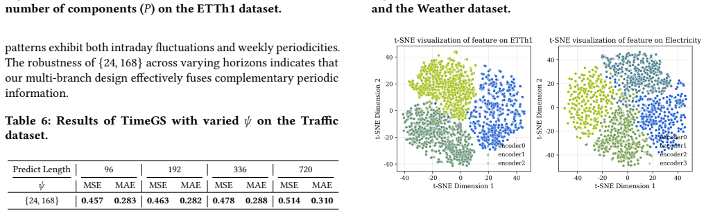
- [§4.2; Table 14; Table 6] The entire pipeline depends on the period-length hyperparameter ψ, which is set manually from domain knowledge (Table 14: ψ=24 for ETTh/Electricity, ψ=96 for ETTm, ψ=144 for Weather, ψ={24,168} for Traffic). The 2D reshape, the anchor positions, and the rasterization all assume this period. If the period is misspecified or the data are aperiodic, the method may inject artificial grid structure. The only sensitivity analysis is Table 6 on Traffic with three ψ configurations, and the differences are modest (e.g., 0.457 vs 0.460 at horizon 96). This is not sufficient to establish robustness across datasets with mixed or unknown periodicities. The authors should either provide an automatic/adaptive period-selection method or report sensitivity analyses for each dataset showing that performance is stable to reasonable ψ misspecification.
- [§4.4, Eqs. (13)–(14)] The theoretical formulation in Eq. (13) defines rendering on an infinite-height 2D plane with a distance function ρ_k that should wrap around period boundaries. The practical implementation in Eq. (14) instead 'symmetrically pads the columns of the kernel with zeros until the total number of columns equals ψ_k' and then flattens and shifts the padded kernel. Zero-padding does not wrap the Gaussian around the grid boundary; it simply truncates the kernel inside a finite window before flattening. As described, the operation is equivalent to placing a finite-support 1D kernel at the target temporal position, not to a chronologically continuous periodic rendering. The claimed 'strict temporal continuity across periodic boundaries' is therefore not demonstrated and may not be realized by the implementation. The authors should provide explicit pseudocode for ρ_k, π_k, and the padding/placement
- [§5.3, Table 4] The ablation on the rendering paradigm does not strongly support the central novelty. Table 4 shows that replacing the Gaussian rendering head with a simple MLP yields almost identical or even better results on several metrics: on Electricity, MLP achieves MSE 0.179 vs Origin 0.181; on Weather, both are 0.245 vs 0.244; on ETTh1, MLP is 0.423 vs 0.419. The claimed 'fundamental advantage of the generative rendering paradigm' is thus not evident from the reported ablation. The authors should either demonstrate settings where rendering clearly helps, or temper the claim that rendering is a paradigm shift rather than an alternative decoder.
minor comments (4)
- [Abstract; Fig. 1 caption] There are several typos: 'intraperiod- fluctuations' and 'interperiod- trends' contain stray hyphens; the Fig. 1 caption says 'may can break'; the abstract says 'state-of-the-art or competitive' while the conclusion says 'state-of-the-art', which should be harmonized.
- [§4.2–§4.4; Table 14] Several important hyperparameters are not specified in the main text or Table 14: the number of Gaussian anchors G, the basis-bank size M, the number of branches K, and the number of components P are mentioned but their chosen values are not reported in a central place. Table 14 lists only ψ, λ, learning rate, and batch size. Please provide a full configuration table.
- [Table 13] The standard deviations in Table 13 are almost all 0.000 or 0.001, which is suspicious for three independent runs on real-world benchmarks. Please clarify the experimental protocol: are these three runs using different seeds? Are the reported MSE values the mean of three runs? If the deviations are truly this small, provide more significant digits; otherwise, the table may mislead readers.
- [General] The paper uses an ACM template with '©2018 Copyright' and '2018' in the reference format, while the arXiv submission is dated 2026. This appears to be a template artifact and should be corrected. Also, the code link should be verified and the repository should contain the exact configuration used for each dataset.
Circularity Check
No circularity found: TimeGS is a supervised learned architecture; no prediction reduces to a fit or self-citation chain.
full rationale
TimeGS is an end-to-end supervised forecasting architecture: the output is a parametric function of the input (UNet features, basis weights/intensities, rasterized Gaussian sums, channel-adaptive fusion) trained by minimizing MSE/MAE against ground truth (Eqs. 10–18). No component of the output is defined in terms of the target, and no parameter is fitted to test labels and then renamed a prediction. The period hyperparameter ψ is chosen from domain knowledge (Table 14), which is a standard modeling inductive bias rather than a fitted quantity; the fixed Gaussian basis bank is frozen, not optimized against the target. The self-citations (PDF [3], TimeBridge [23], FinMamba [9], etc.) appear only in related-work or motivation contexts and are not load-bearing: the 2D period-phase motivation is independently supported by TimesNet [42], and the central rendering claim does not rest on any of the authors' prior results. No uniqueness theorem is invoked, and no known empirical pattern is merely renamed. The Table 1 discrepancy between the abstract's SOTA wording and the reported baseline numbers on several datasets is an empirical-support/correctness concern, not a circularity concern.
Axiom & Free-Parameter Ledger
free parameters (8)
- Period length ψ =
{24}, {96}, {144}, {24,168}
- Number of branches K =
not reported (grid-searched)
- Number of components P =
not reported (grid-searched)
- Loss weight λ =
0.5 (0.0 for ETTh2)
- Learning rate =
1e-3 or 1e-4
- Batch size =
16 or 32
- Gaussian basis bank size M / shapes =
not specified
- Anchor positions G =
not specified
axioms (5)
- domain assumption Each dataset has a fixed dominant period ψ, and folding the series into rows of length ψ exposes the intraperiod/interperiod structure (Section 4.2).
- ad hoc to paper The future sequence can be represented as a weighted sum of a fixed set of Gaussian kernels at fixed anchor positions (Eq 13-14).
- ad hoc to paper The flattened/padded rasterization exactly implements rendering on an infinite-height 2D temporal plane (§4.4 Practical Implementation).
- domain assumption Channel-independent processing with shared parameters is beneficial (Section 4.1).
- ad hoc to paper The frozen Gaussian basis bank is sufficiently expressive to represent local variations (Section 4.3).
read the original abstract
Time series forecasting remains a challenging problem due to the intricate entanglement of intra-period fluctuations and inter-period trends. While recent advances have attempted to reshape 1D sequences into 2D period-phase representations, they suffer from two principal limitations. Firstly, treating reshaped tensors as static images results in a topological mismatch, as standard spatial operators sever chronological continuity at grid boundaries. Secondly, relying on uniform fixed-size representations allocates modeling capacity inefficiently and fails to provide the adaptive resolution required for compressible, non-stationary temporal patterns. To address these limitations, we introduce TimeGS, a novel framework that fundamentally shifts the forecasting paradigm from regression to 2D generative rendering. By reconceptualizing the future sequence as a latent 2D temporal surface, TimeGS utilizes the inherent anisotropy of Gaussian kernels to adaptively model complex variations with flexible geometric alignment. To realize this, we introduce a Multi-Basis Gaussian Kernel Generation (MB-GKG) block that synthesizes kernels from a fixed dictionary to stabilize optimization, and a Multi-Period Chronologically Continuous Rasterization (MP-CCR) block that enforces strict temporal continuity across periodic boundaries. Comprehensive experiments on standard benchmark datasets demonstrate that TimeGS attains state-of-the-art or competitive performance. The code is at https://github.com/yixinwang1/TimeGS.
Figures




Reference graph
Works this paper leans on
-
[1]
Michal Aharon, Michael Elad, and Alfred Bruckstein. 2006. K-SVD: An algo- rithm for designing overcomplete dictionaries for sparse representation.IEEE Transactions on signal processing54, 11 (2006), 4311–4322
2006
-
[2]
Cristian Challu, Kin G Olivares, Boris N Oreshkin, Federico Garza, Max Mergen- thaler, and Artur Dubrawski. 2023. N-HiTS: Neural Hierarchical Interpolation for Time Series Forecasting.AAAI(2023)
2023
-
[3]
Tao Dai, Beiliang Wu, Peiyuan Liu, Naiqi Li, Jigang Bao, Yong Jiang, and Shu-Tao Xia. 2024. Periodicity Decoupling Framework for Long-term Series Forecasting. International Conference on Learning Representations(2024)
2024
-
[4]
Chirag Deb, Fan Zhang, Junjing Yang, Siew Eang Lee, and Kwok Wei Shah. 2017. A review on time series forecasting techniques for building energy consumption. Renewable and Sustainable Energy Reviews74 (2017), 902–924
2017
-
[5]
Jiajun Dong, Chengkun Wang, Wenzhao Zheng, Lei Chen, Jiwen Lu, and Yansong Tang. 2025. Gaussiantoken: An effective image tokenizer with 2d gaussian splatting.arXiv preprint arXiv:2501.15619(2025)
Pith/arXiv arXiv 2025
-
[6]
Lu Han, Han-Jia Ye, and De-Chuan Zhan. 2024. The capacity and robustness trade-off: Revisiting the channel independent strategy for multivariate time series forecasting.IEEE Transactions on Knowledge and Data Engineering36, 11 (2024), 7129–7142
2024
-
[7]
Pradeep Hewage, Ardhendu Behera, Marcello Trovati, Ella Pereira, Morteza Ghahremani, Francesco Palmieri, and Yonghuai Liu. 2020. Temporal convolutional neural (TCN) network for an effective weather forecasting using time-series data from the local weather station.Soft Computing24, 21 (2020), 16453–16482
2020
-
[8]
Jintong Hu, Bin Xia, Bin Chen, Wenming Yang, and Lei Zhang. 2025. Gaussiansr: High fidelity 2d gaussian splatting for arbitrary-scale image super-resolution. In Proceedings of the AAAI Conference on Artificial Intelligence, Vol. 39. 3554–3562
2025
-
[9]
Yifan Hu, Peiyuan Liu, Yuante Li, Dawei Cheng, Naiqi Li, Tao Dai, Jigang Bao, and Xia Shu-Tao. 2025. FinMamba: Market-Aware Graph Enhanced Multi-Level Mamba for Stock Movement Prediction.arXiv preprint arXiv:2502.06707(2025)
Pith/arXiv arXiv 2025
-
[10]
Yifan Hu, Peiyuan Liu, Peng Zhu, Dawei Cheng, and Tao Dai. 2025. Adaptive multi-scale decomposition framework for time series forecasting. InProceedings of the AAAI Conference on Artificial Intelligence, Vol. 39. 17359–17367
2025
-
[11]
Yifan Hu, Jie Yang, Tian Zhou, Peiyuan Liu, Yujin Tang, Rong Jin, and Liang Sun
-
[12]
Yifan Hu, Guibin Zhang, Peiyuan Liu, Disen Lan, Naiqi Li, Dawei Cheng, Tao Dai, Shu-Tao Xia, and Shirui Pan. 2025. TimeFilter: Patch-Specific Spatial-Temporal Graph Filtration for Time Series Forecasting. InForty-second International Con- ference on Machine Learning. https://openreview.net/forum?id=490VcNtjh7
2025
-
[13]
Binbin Huang, Zehao Yu, Anpei Chen, Andreas Geiger, and Shenghua Gao
-
[14]
Qihe Huang, Zhengyang Zhou, Kuo Yang, Zhongchao Yi, Xu Wang, and Yang Wang. 2025. TimeBase: The Power of Minimalism in Efficient Long-term Time Series Forecasting. InForty-second International Conference on Machine Learning. https://openreview.net/forum?id=GhTdNOMfOD
2025
-
[15]
Peter J Huber. 1992. Robust estimation of a location parameter. InBreakthroughs in statistics: Methodology and distribution. Springer, 492–518
1992
-
[16]
Zahra Karevan and Johan AK Suykens. 2020. Transductive LSTM for time-series prediction: An application to weather forecasting.Neural Networks125 (2020), 1–9
2020
-
[17]
Bernhard Kerbl, Georgios Kopanas, Thomas Leimkühler, and George Drettakis
-
[18]
Taesung Kim, Jinhee Kim, Yunwon Tae, Cheonbok Park, Jang-Ho Choi, and Jaegul Choo. 2021. Reversible instance normalization for accurate time-series forecasting against distribution shift. InInternational conference on learning representations
2021
-
[19]
Kingma and Jimmy Ba
Diederik P. Kingma and Jimmy Ba. 2015. Adam: A Method for Stochastic Opti- mization.ICLR(2015)
2015
-
[20]
Hongyu Li, Chaofeng Chen, Xiaoming Li, and Guangming Lu. 2025. 2D Gauss- ian Splatting with Semantic Alignment for Image Inpainting.arXiv preprint arXiv:2509.01964(2025)
Pith/arXiv arXiv 2025
-
[21]
Bryan Lim, Sercan Ö Arık, Nicolas Loeff, and Tomas Pfister. 2021. Temporal fusion transformers for interpretable multi-horizon time series forecasting.International journal of forecasting37, 4 (2021), 1748–1764
2021
-
[22]
Shengsheng Lin, Weiwei Lin, Xinyi Hu, Wentai Wu, Ruichao Mo, and Haocheng Zhong. 2024. Cyclenet: Enhancing time series forecasting through modeling periodic patterns.Advances in Neural Information Processing Systems37 (2024), 106315–106345
2024
-
[23]
Peiyuan Liu, Beiliang Wu, Yifan Hu, Naiqi Li, Tao Dai, Jigang Bao, and Shu- tao Xia. 2024. Timebridge: Non-stationarity matters for long-term time series forecasting.arXiv preprint arXiv:2410.04442(2024)
Pith/arXiv arXiv 2024
-
[24]
Shizhan Liu, Hang Yu, Cong Liao, Jianguo Li, Weiyao Lin, Alex X Liu, and Schahram Dustdar. 2021. Pyraformer: Low-complexity pyramidal attention for long-range time series modeling and forecasting.ICLR(2021)
2021
-
[25]
Yong Liu, Tengge Hu, Haoran Zhang, Haixu Wu, Shiyu Wang, Lintao Ma, and Mingsheng Long. [n. d.]. iTransformer: Inverted Transformers Are Effective for Time Series Forecasting. InThe Twelfth International Conference on Learning Representations
-
[26]
Laurens van der Maaten and Geoffrey Hinton. 2008. Visualizing data using t-SNE. Journal of machine learning research9, Nov (2008), 2579–2605
2008
-
[27]
Md Mahmuddun Nabi Murad, Mehmet Aktukmak, and Yasin Yilmaz. 2025. Wp- mixer: Efficient multi-resolution mixing for long-term time series forecasting. In Proceedings of the AAAI Conference on Artificial Intelligence, Vol. 39. 19581–19588
2025
-
[28]
Reza Nematirad, Anil Pahwa, and Balasubramaniam Natarajan. 2025. Times2d: Multi-period decomposition and derivative mapping for general time series forecasting. InProceedings of the AAAI Conference on Artificial Intelligence, Vol. 39. 19651–19658
2025
-
[29]
Yuqi Nie, Nam H Nguyen, Phanwadee Sinthong, and Jayant Kalagnanam. 2023. A Time Series is Worth 64 Words: Long-term Forecasting with Transformers. ICLR(2023)
2023
-
[30]
Henri J Nussbaumer. 1981. The fast Fourier transform. InFast Fourier transform and convolution algorithms. Springer, 80–111
1981
-
[31]
Boris N Oreshkin, Dmitri Carpov, Nicolas Chapados, and Yoshua Bengio. 2019. N- BEATS: Neural basis expansion analysis for interpretable time series forecasting. ICLR(2019)
2019
-
[32]
Adam Paszke, Sam Gross, Francisco Massa, Adam Lerer, James Bradbury, Gregory Chanan, Trevor Killeen, Zeming Lin, Natalia Gimelshein, Luca Antiga, et al. 2019. Pytorch: An imperative style, high-performance deep learning library.Advances in neural information processing systems32 (2019)
2019
-
[33]
Xiangfei Qiu, Xingjian Wu, Yan Lin, Chenjuan Guo, Jilin Hu, and Bin Yang
-
[34]
Olaf Ronneberger, Philipp Fischer, and Thomas Brox. 2015. U-net: Convolutional networks for biomedical image segmentation. InInternational Conference on Medical image computing and computer-assisted intervention. Springer, 234–241
2015
-
[35]
Diaa Salman, Cem Direkoglu, Mehmet Kusaf, and Murat Fahrioglu. 2024. Hybrid deep learning models for time series forecasting of solar power.Neural Computing and Applications36, 16 (2024), 9095–9112
2024
-
[36]
Omer Berat Sezer, Mehmet Ugur Gudelek, and Ahmet Murat Ozbayoglu. 2020. Financial time series forecasting with deep learning: A systematic literature review: 2005–2019.Applied soft computing90 (2020), 106181
2020
-
[37]
In SIGKDD
DUET: Dual Clustering Enhanced Multivariate Time Series Forecasting. In SIGKDD. 1185–1196
-
[38]
Haotian Si, Changhua Pei, Jianhui li, Dan Pei, and Gaogang Xie. 2025. CMoS: Rethinking Time Series Prediction Through the Lens of Chunk-wise Spatial Correlations. InForty-second International Conference on Machine Learning. https: //openreview.net/forum?id=eyjrms4HHm
2025
-
[39]
Huiqiang Wang, Jian Peng, Feihu Huang, Jince Wang, Junhui Chen, and Yifei Xiao. 2023. MICN: Multi-scale Local and Global Context Modeling for Long-term Series Forecasting.ICLR(2023)
2023
-
[40]
Zhang, and JUN ZHOU
Shiyu Wang, Haixu Wu, Xiaoming Shi, Tengge Hu, Huakun Luo, Lintao Ma, James Y. Zhang, and JUN ZHOU. 2024. TimeMixer: Decomposable Multiscale Mixing for Time Series Forecasting. InThe Twelfth International Conference on Learning Representations. https://openreview.net/forum?id=7oLshfEIC2
2024
-
[41]
Noam Shazeer, Azalia Mirhoseini, Krzysztof Maziarz, Andy Davis, Quoc Le, Geoffrey Hinton, and Jeff Dean. 2017. Outrageously large neural networks: The sparsely-gated mixture-of-experts layer.arXiv preprint arXiv:1701.06538(2017)
Pith/arXiv arXiv 2017
-
[42]
Haixu Wu, Tengge Hu, Yong Liu, Hang Zhou, Jianmin Wang, and Mingsheng Long. 2023. TimesNet: Temporal 2D-Variation Modeling for General Time Series Analysis.ICLR(2023)
2023
-
[43]
Haixu Wu, Jiehui Xu, Jianmin Wang, and Mingsheng Long. 2021. Autoformer: Decomposition Transformers with Auto-Correlation for Long-Term Series Fore- casting.NeurIPS(2021)
2021
-
[44]
Zhijian Xu, Ailing Zeng, and Qiang Xu. 2023. FITS: Modeling time series with 10𝑘parameters.arXiv preprint arXiv:2307.03756(2023)
Pith/arXiv arXiv 2023
-
[45]
Yuxuan Wang, Haixu Wu, Jiaxiang Dong, Yong Liu, Chen Wang, Mingsheng Long, and Jianmin Wang. 2024. Deep time series models: A comprehensive survey and benchmark.arXiv preprint arXiv:2407.13278(2024)
Pith/arXiv arXiv 2024
-
[46]
Xinjie Zhang, Xingtong Ge, Tongda Xu, Dailan He, Yan Wang, Hongwei Qin, Guo Lu, Jing Geng, and Jun Zhang. 2024. Gaussianimage: 1000 fps image repre- sentation and compression by 2d gaussian splatting. InEuropean Conference on Computer Vision. Springer, 327–345
2024
-
[47]
Yunhao Zhang and Junchi Yan. 2023. Crossformer: Transformer utilizing cross- dimension dependency for multivariate time series forecasting.ICLR(2023)
2023
-
[48]
Haoyi Zhou, Shanghang Zhang, Jieqi Peng, Shuai Zhang, Jianxin Li, Hui Xiong, and Wancai Zhang. 2021. Informer: Beyond Efficient Transformer for Long Sequence Time-Series Forecasting.AAAI(2021)
2021
-
[49]
Ailing Zeng, Muxi Chen, Lei Zhang, and Qiang Xu. 2023. Are transformers effective for time series forecasting?AAAI(2023)
2023
-
[53]
Tian Zhou, Ziqing Ma, Qingsong Wen, Xue Wang, Liang Sun, and Rong Jin. 2022. FEDformer: Frequency enhanced decomposed transformer for long-term series forecasting.ICML(2022). arXiv Preprint, February, 2026 A Dataset We evaluate TimeGS on multiple standard time series benchmarks for long-term forecasting. Table 8 provides detailed descriptions of their cha...
2022
-
[2023]
Graph.42, 4 (2023), 139–1
3D Gaussian splatting for real-time radiance field rendering.ACM Trans. Graph.42, 4 (2023), 139–1
2023
-
[2024]
InACM SIGGRAPH 2024 conference papers
2d gaussian splatting for geometrically accurate radiance fields. InACM SIGGRAPH 2024 conference papers. 1–11
2024
-
[2025]
Bridging Past and Future: Distribution-Aware Alignment for Time Series Forecasting.arXiv preprint arXiv:2509.14181(2025)
arXiv 2025
discussion (0)
Sign in with ORCID, Apple, or X to comment. Anyone can read and Pith papers without signing in.