Recognition: unknown
Reconstructing inflationary features on large scales using genetic algorithm
Pith reviewed 2026-05-10 12:48 UTC · model grok-4.3
The pith
A genetic algorithm can reconstruct modifications to the slow-roll parameter that generate features in the primordial power spectrum and improve the fit to Planck CMB data by Delta chi-squared of at least 10.
A machine-rendered reading of the paper's core claim, the machinery that carries it, and where it could break.
Core claim
By using a genetic algorithm to evolve the functional form of the first slow-roll parameter around a baseline slow-rolling model, the authors generate scalar power spectra containing localized features. These spectra improve the fit to the Planck 2018 angular power spectra by a Delta chi-squared of at most minus 10. The same algorithm also locates alternative sets of background parameters paired with different features that deliver similar fit improvements, all while providing effective single-field inflationary dynamics consistent with the data.
What carries the argument
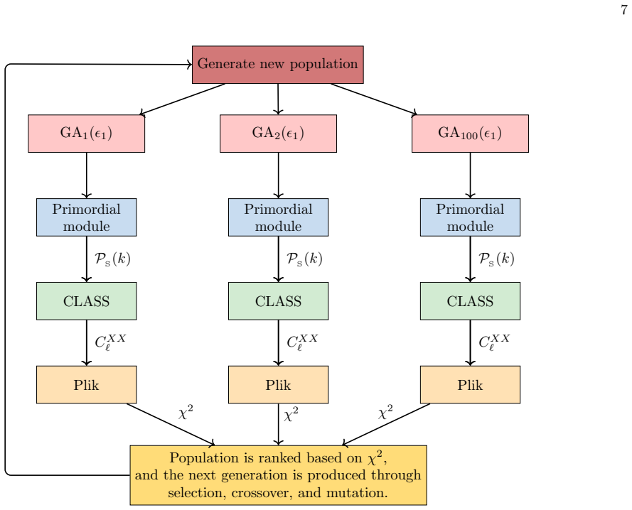
The genetic algorithm that evolves modifications to the time-dependent first slow-roll parameter to optimize the match between the generated primordial power spectrum and the observed CMB anisotropies.
Load-bearing premise
The modifications to the slow-roll parameter remain consistent with the slow-roll approximation and can be realized in a canonical single-field potential when the background LambdaCDM parameters are held at their standard values derived from a featureless spectrum.
What would settle it
Independent data from future CMB polarization measurements or large-scale structure surveys that show no improvement or a worse fit when using the reconstructed power spectra would indicate that the features are not supported by observations.
Figures


read the original abstract
[Abridged] A variety of model-dependent as well as model-independent approaches suggest that certain localized features in the primordial scalar power spectrum can lead to a significantly better fit to the observed anisotropies in the cosmic microwave background (CMB). In this work, we focus on three types of such features and examine whether these features can be generated in inflationary scenarios driven by a single, canonical scalar field. We consider a slowly rolling baseline model that is described by a specific time-dependence of the first slow roll parameter and we generate the desired features in the power spectrum through suitable modifications to the functional form of the slow roll parameter. To systematically reconstruct the desired features in the scalar power spectrum (or, equivalently, the modifications in the behavior of the first slow roll parameter) that are consistent with the data, we implement a machine learning pipeline based on the genetic algorithm (GA). Assuming the standard values for the background $\Lambda$CDM model (arrived at for a nearly scale-invariant primordial scalar power spectrum), we apply our method to the Planck 2018 CMB data, and show that the reconstructed features improve the fit to the observed angular power spectra by $\Delta \chi^2 \lesssim -10$. Moreover, we find that GA points to other sets of background parameters and primordial features, which lead to a similar level of improvement in the fit to the data. Such alternative sets of background parameters and scalar power spectra offer possible pathways to alleviate existing cosmological tensions. Our approach provides effective single-field inflationary dynamics to generate features that are supported by the data.
Editorial analysis
A structured set of objections, weighed in public.
Referee Report
Summary. The paper uses a genetic algorithm (GA) to reconstruct localized modifications to the first slow-roll parameter ε(N) starting from a baseline slow-roll model, generating features in the primordial scalar power spectrum P(k) that are then compared to Planck 2018 CMB angular power spectra. It reports that these GA-optimized features improve the fit by Δχ² ≲ -10 relative to the standard nearly scale-invariant case, while also identifying alternative background parameter sets that achieve comparable improvements and may help alleviate cosmological tensions. The approach is presented as providing effective single-field inflationary dynamics consistent with the data.
Significance. If the reconstructed ε(N) modifications can be shown to integrate to a canonical single-field potential while preserving the slow-roll regime and the validity of the power-spectrum formula used for the fit, the work would offer a systematic, data-driven method for identifying viable feature-generating inflationary models. The identification of multiple alternative background+feature combinations with similar Δχ² gains is a potentially useful contribution for exploring tensions, provided the GA results are validated against overfitting and convergence issues.
major comments (3)
- [reconstruction method and results] The central claim that the GA-reconstructed modifications to ε(N) remain realizable in canonical single-field inflation requires explicit verification that the second slow-roll parameter η remains ≪1 over the relevant range of e-folds. The manuscript applies the standard slow-roll power-spectrum formula to compute the fit but does not integrate the optimized ε(N) back to V(φ) via dφ/dN = −√(2ε) and V = 3H²(1−ε), nor does it report checks on η = (1/2)d ln ε/dN + ε. This is load-bearing for the single-field interpretation (see abstract and the reconstruction pipeline description).
- [GA implementation and application to Planck data] No details are provided on GA convergence, population size, mutation/crossover rates, number of independent runs, or validation against overfitting (e.g., via cross-validation or comparison to mock data with known features). The reported Δχ² ≲ -10 is obtained by direct optimization against the same Planck data used to define the target, so quantitative assessment of robustness is needed to support the claim of data-supported features.
- [results on alternative parameter sets] Error estimation on the reconstructed features and background parameters is not described. Without posterior uncertainties or bootstrap-style errors on the GA solutions, it is unclear whether the alternative background+feature sets are statistically distinguishable from the baseline or from each other.
minor comments (2)
- [abstract and results] The abstract states 'Δχ² ≲ -10' but the precise value, the number of degrees of freedom, and the baseline model against which the improvement is measured should be stated explicitly in the results section for reproducibility.
- [method] Notation for the functional form of the slow-roll modification and the GA hyperparameters should be defined in a dedicated subsection or table to improve clarity.
Simulated Author's Rebuttal
We thank the referee for the careful and constructive review. The comments identify important gaps in verification, implementation details, and uncertainty quantification. We have revised the manuscript to address each point directly, adding the requested calculations, GA specifications, and error estimates while preserving the original results and interpretations.
read point-by-point responses
-
Referee: The central claim that the GA-reconstructed modifications to ε(N) remain realizable in canonical single-field inflation requires explicit verification that the second slow-roll parameter η remains ≪1 over the relevant range of e-folds. The manuscript applies the standard slow-roll power-spectrum formula to compute the fit but does not integrate the optimized ε(N) back to V(φ) via dφ/dN = −√(2ε) and V = 3H²(1−ε), nor does it report checks on η = (1/2)d ln ε/dN + ε. This is load-bearing for the single-field interpretation (see abstract and the reconstruction pipeline description).
Authors: We agree that explicit verification of the slow-roll regime is necessary to substantiate the single-field interpretation. In the revised manuscript we have added a dedicated subsection that integrates each optimized ε(N) to obtain the corresponding inflaton potential via dφ/dN = −√(2ε) and V(φ) = 3H²(1−ε). We then compute η(N) = (1/2) d ln ε/dN + ε and demonstrate that |η| remains ≪ 1 throughout the relevant e-fold range for all reported solutions. These checks confirm that the slow-roll power-spectrum formula remains valid and that the reconstructed features are realizable within canonical single-field inflation. revision: yes
-
Referee: No details are provided on GA convergence, population size, mutation/crossover rates, number of independent runs, or validation against overfitting (e.g., via cross-validation or comparison to mock data with known features). The reported Δχ² ≲ -10 is obtained by direct optimization against the same Planck data used to define the target, so quantitative assessment of robustness is needed to support the claim of data-supported features.
Authors: We appreciate the request for implementation transparency. The revised manuscript now contains a new subsection that specifies the GA hyperparameters (population size 200, mutation probability 0.05, crossover probability 0.9, 50 generations) and reports results from 20 independent runs with distinct random seeds. All runs converge to solutions with Δχ² ≲ −10. To assess overfitting we have added recovery tests on mock Planck-like spectra containing known localized features; the GA reliably reconstructs the injected features while avoiding spurious ones, thereby supporting the robustness of the reported improvements. revision: yes
-
Referee: Error estimation on the reconstructed features and background parameters is not described. Without posterior uncertainties or bootstrap-style errors on the GA solutions, it is unclear whether the alternative background+feature sets are statistically distinguishable from the baseline or from each other.
Authors: We acknowledge that quantitative uncertainties were omitted from the original submission. In the revision we have implemented a bootstrap procedure: the Planck likelihood is resampled 100 times and the GA is re-run on each realization. The resulting ensemble yields 1σ uncertainties on both the reconstructed ε(N) features and the background parameters. These uncertainties are now shown in updated figures and tables. The analysis indicates that while some alternative background+feature combinations lie within the bootstrap errors of the baseline, others remain distinguishable and continue to offer viable pathways for alleviating cosmological tensions. revision: yes
Circularity Check
GA optimization of ε(N) modifications reports Δχ² improvement by construction against Planck data
specific steps
-
fitted input called prediction
[Abstract]
"Assuming the standard values for the background ΛCDM model (arrived at for a nearly scale-invariant primordial scalar power spectrum), we apply our method to the Planck 2018 CMB data, and show that the reconstructed features improve the fit to the observed angular power spectra by Δχ² ≲ -10. Moreover, we find that GA points to other sets of background parameters and primordial features, which lead to a similar level of improvement in the fit to the data."
The genetic algorithm is explicitly used to reconstruct modifications to ε(N) that minimize the mismatch with the Planck data; therefore the quoted Δχ² improvement and the discovery of alternative parameter sets are the direct numerical outcome of the optimization against the target dataset rather than an a priori prediction or first-principles result.
full rationale
The paper's core result uses a genetic algorithm to optimize localized modifications to the first slow-roll parameter ε(N) (starting from a baseline slow-roll model) in order to generate features in the scalar power spectrum that better match the Planck 2018 CMB angular power spectra. The reported improvement Δχ² ≲ -10 is the direct output of this data-driven optimization, and the additional finding of alternative background parameters yielding similar fits is likewise produced by the same fitting procedure. While the method transparently reconstructs features and assumes consistency with single-field slow-roll dynamics, the quantitative claim of improved fit reduces to the optimization target itself rather than an independent derivation or prediction. No self-citation chains, uniqueness theorems, or smuggled ansatzes appear in the provided text, so circularity is limited to the fitted-input pattern and remains partial.
Axiom & Free-Parameter Ledger
free parameters (2)
- parameters controlling the functional form of the slow-roll modification
- genetic algorithm hyperparameters
axioms (2)
- domain assumption Features in the primordial scalar power spectrum can be produced by modifications to the first slow-roll parameter in single-field canonical inflation
- domain assumption Standard ΛCDM background parameters provide a valid baseline
Reference graph
Works this paper leans on
-
[1]
(Later, we shall consider another set of background parameters for DOGE
In the DOGE scenario Let us first consider the case wherein the baseline first slow roll parameter is modified by DOGE. (Later, we shall consider another set of background parameters for DOGE. Therefore, for convenience, we shall refer to this case as DOGE I.) In this case, we obtain the minimum value of the goodness of fit to beχ 2 = 2760.51. This corres...
-
[2]
(21) In Fig
In the CPSC model For the type of features generated by the CPSC mod- els, the functionF(N) that leads to the best-fit to the Planck 2018 data, as constructed by GA, turns out to be F(N) =−0.009 tanh[N−16.81] 1 + 0.99(N−16.81) 2 + 0.003 e−(N−18.28) 2 sin[10.09(N−18.28)] −0.009 tanh[N−16.84] 1 + 0.99(N−16.84) 2 + 0.002 e−(N−17.96) 2 sin[18.43(N−17.96)]. (2...
2018
-
[3]
(18) and (19), along with the priors listed in Tab
In the MRL case To emulate features indicated by the MRL reconstruc- tions, we employ a GA run using theF(N) in Eqs. (18) and (19), along with the priors listed in Tab. III. We find the best-fitF(N) to be F(N) = 1−tanh N−14.23 0.22 + 0.042 1.0 + 1.09 1 + 342.14(N−14.80) 2 + 0.048 1.0 + 0.62 sin 262.95(N−13.03) 1 + 31(N−13.03) 2 + 1−tanh N−14.32 0.40 + 0.0...
2018
-
[4]
V. F. Mukhanov, H. A. Feldman, and R. H. Branden- berger, Phys. Rept.215, 203 (1992)
1992
- [5]
- [6]
-
[7]
B. A. Bassett, S. Tsujikawa, and D. Wands, Rev. Mod. Phys.78, 537 (2006)
2006
-
[8]
An introduction to inflation and cosmological perturbation theory
L. Sriramkumar, Curr. Sci.97, 868 (2009), arXiv:0904.4584 [astro-ph.CO]
-
[9]
D. Baumann and H. V. Peiris, Adv. Sci. Lett.2, 105 (2009), arXiv:0810.3022 [astro-ph]
-
[10]
D. Baumann, inPhysics of the Large and the Small scales(2011) pp. 523–686, arXiv:0907.5424 [hep-th]
work page Pith review arXiv 2011
-
[11]
On the generation and evolution of perturbations during inflation and reheating,
L. Sriramkumar, “On the generation and evolution of perturbations during inflation and reheating,” inVi- gnettes in Gravitation and Cosmology, edited by L. Sri- ramkumar and T. R. Seshadri (2012) pp. 207–249
2012
-
[12]
Inflationary cosmology after planck 2013.arXiv preprint arXiv:1402.0526, 2014
A. Linde, inPost-Planck Cosmology(2014) arXiv:1402.0526 [hep-th]
-
[13]
J. Martin, Astrophys. Space Sci. Proc.45, 41 (2016), arXiv:1502.05733 [astro-ph.CO]
-
[14]
Planck 2018 results. X. Constraints on inflation
Y. Akramiet al.(Planck), Astron. Astrophys.641, A10 (2020), arXiv:1807.06211 [astro-ph.CO]
work page internal anchor Pith review arXiv 2020
-
[15]
Planck 2018 results. IX. Constraints on primordial non-Gaussianity
Y. Akramiet al.(Planck), Astron. Astrophys.641, A9 (2020), arXiv:1905.05697 [astro-ph.CO]
work page Pith review arXiv 2020
- [16]
-
[17]
Campetiet al.(LiteBIRD), JCAP06, 008 (2024), arXiv:2312.00717 [astro-ph.CO]
P. Campetiet al.(LiteBIRD), JCAP06, 008 (2024), arXiv:2312.00717 [astro-ph.CO]
-
[18]
T. Ghignaet al.(LiteBIRD), inSPIE Astro- nomical Telescopes + Instrumentation 2024(2024) arXiv:2406.02724 [astro-ph.IM]
-
[19]
Y. Mellieret al.(Euclid), Astron. Astrophys.697, A1 (2025), arXiv:2405.13491 [astro-ph.CO]
- [20]
-
[21]
E. Camphuiset al.(SPT-3G), (2025), arXiv:2506.20707 [astro-ph.CO]
work page internal anchor Pith review arXiv 2025
-
[22]
arXive-prints, arXiv:2503.00636doi:10
M. Abitbolet al.(Simons Observatory), JCAP08, 034 (2025), arXiv:2503.00636 [astro-ph.IM]
- [23]
- [24]
- [25]
-
[26]
Ballardiniet al.(Euclid), Astron
M. Ballardiniet al.(Euclid), Astron. Astrophys.683, A220 (2024), arXiv:2309.17287 [astro-ph.CO]
- [27]
- [28]
- [29]
-
[30]
A. Shafieloo and T. Souradeep, Phys. Rev. D70, 043523 (2004), arXiv:astro-ph/0312174
-
[31]
A. Shafieloo, T. Souradeep, P. Manimaran, P. K. Pan- igrahi, and R. Rangarajan, Phys. Rev. D75, 123502 (2007), arXiv:astro-ph/0611352
-
[32]
A. Shafieloo and T. Souradeep, Phys. Rev. D78, 023511 (2008), arXiv:0709.1944 [astro-ph]
- [33]
-
[34]
G. Nicholson and C. R. Contaldi, JCAP07, 011 (2009), arXiv:0903.1106 [astro-ph.CO]
-
[35]
G. Nicholson, C. R. Contaldi, and P. Paykari, JCAP 01, 016 (2010), arXiv:0909.5092 [astro-ph.CO]
- [36]
- [37]
- [38]
- [39]
- [40]
- [41]
- [42]
-
[43]
M. Braglia, X. Chen, and D. K. Hazra, Phys. Rev. D 105, 103523 (2022), arXiv:2108.10110 [astro-ph.CO]
- [44]
- [45]
-
[46]
N. Sch¨ oneberg, G. Franco Abell´ an, A. P´ erez S´ anchez, S. J. Witte, V. Poulin, and J. Lesgourgues, Phys. Rept. 984, 1 (2022), arXiv:2107.10291 [astro-ph.CO]
-
[47]
W. H. Richardson, J. Opt. Soc. Am.62, 55 (1972)
1972
-
[48]
Weinberg,Cosmology(Oxford University Press, Ox- ford, England, 2008)
S. Weinberg,Cosmology(Oxford University Press, Ox- ford, England, 2008)
2008
-
[49]
Dodelson and F
S. Dodelson and F. Schmidt,Modern Cosmology(Aca- demic Press, London, England, 2020)
2020
-
[50]
Durrer,The Cosmic Microwave Background(Cam- bridge University Press, Cambridge, England, 2020)
R. Durrer,The Cosmic Microwave Background(Cam- bridge University Press, Cambridge, England, 2020)
2020
-
[51]
N. Aghanimet al.(Planck), Astron. Astrophys.641, A5 (2020), arXiv:1907.12875 [astro-ph.CO]
-
[52]
The Cosmic Linear Anisotropy Solving System (CLASS) I: Overview
J. Lesgourgues, (2011), arXiv:1104.2932 [astro-ph.IM]
work page Pith review arXiv 2011
-
[53]
D. Blas, J. Lesgourgues, and T. Tram, JCAP07, 034 (2011), arXiv:1104.2933 [astro-ph.CO]
work page internal anchor Pith review arXiv 2011
- [54]
-
[55]
T. S. Bunch and P. C. W. Davies, Proc. Roy. Soc. Lond. A357, 381 (1977)
1977
-
[56]
T. S. Bunch and P. C. W. Davies, Proc. Roy. Soc. Lond. A360, 117 (1978)
1978
-
[57]
T. S. Bunch and P. C. W. Davies, J. Phys. A11, 1315 (1978)
1978
- [58]
-
[59]
Affenzeller, S
M. Affenzeller, S. Winkler, S. Wagner, and A. Beham, Genetic Algorithms and Genetic Programming(2009)
2009
-
[60]
Mitchell,An Introduction to Genetic Algorithms (MIT Press, Cambridge, MA, USA, 1998)
M. Mitchell,An Introduction to Genetic Algorithms (MIT Press, Cambridge, MA, USA, 1998)
1998
-
[61]
Genetic Algorithms and Supernovae Type Ia Analysis
C. Bogdanos and S. Nesseris, JCAP05, 006 (2009), arXiv:0903.2805 [astro-ph.CO]
work page Pith review arXiv 2009
-
[62]
S. Nesseris and J. Garcia-Bellido, JCAP11, 033 (2012), arXiv:1205.0364 [astro-ph.CO]
-
[63]
R. Arjona and S. Nesseris, Phys. Rev. D101, 123525 (2020), arXiv:1910.01529 [astro-ph.CO]
-
[64]
R. Arjona and S. Nesseris, JCAP11, 042 (2020), arXiv:2001.11420 [astro-ph.CO]
-
[65]
A. Kamerkar, S. Nesseris, and L. Pinol, Phys. Rev. D 108, 043509 (2023), arXiv:2211.14142 [astro-ph.CO]
-
[66]
K. Lodha, L. Pinol, S. Nesseris, A. Shafieloo, W. Sohn, and M. Fasiello, Mon. Not. Roy. Astron. Soc.530, 1424 (2024), arXiv:2308.04940 [astro-ph.CO]
-
[67]
R. Medel-Esquivel, I. G´ omez-Vargas, A. A. M. S´ anchez, R. Garc´ ıa-Salcedo, and J. Alberto V´ azquez, Universe 10, 11 (2024), arXiv:2311.05699 [astro-ph.CO]
-
[68]
Bogdanos and S
C. Bogdanos and S. Nesseris, Journal of Cosmology and Astroparticle Physics2009, 006 (2009)
2009
-
[69]
D. E. Goldberg,Genetic Algorithms and Machine Learning(Addison-Wesley, New York, 1989)
1989
-
[70]
Michalewicz, inSpringer Berlin Heidelberg(1996)
Z. Michalewicz, inSpringer Berlin Heidelberg(1996)
1996
- [71]
- [72]
- [73]
-
[74]
Z.-Y. Peng and Y.-S. Piao, (2025), arXiv:2507.17276 [astro-ph.CO]
-
[75]
M. Braglia, D. K. Hazra, L. Sriramkumar, and F. Finelli, JCAP08, 025 (2020), arXiv:2004.00672 [astro-ph.CO]
- [76]
- [77]
-
[78]
Ichiki and R
K. Ichiki and R. Nagata, Phys. Rev. D80, 083002 (2009)
2009
-
[79]
P. Hunt and S. Sarkar, JCAP01, 025 (2014), arXiv:1308.2317 [astro-ph.CO]
- [80]
discussion (0)
Sign in with ORCID, Apple, or X to comment. Anyone can read and Pith papers without signing in.