Controlled Chaos in 4D SCFTs
Pith reviewed 2026-06-26 07:04 UTC · model grok-4.3
The pith
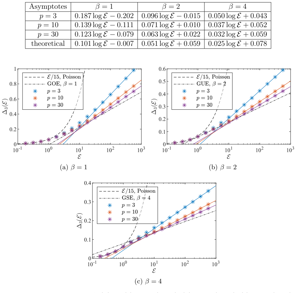
Tuning marginal couplings in orbifold 4D SCFTs produces a chaotic spectrum in the dilatation operator, diagnosed by eigenvalue level repulsion and spectral rigidity.
A machine-rendered reading of the paper's core claim, the machinery that carries it, and where it could break.
Core claim
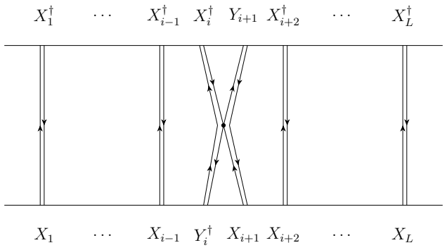
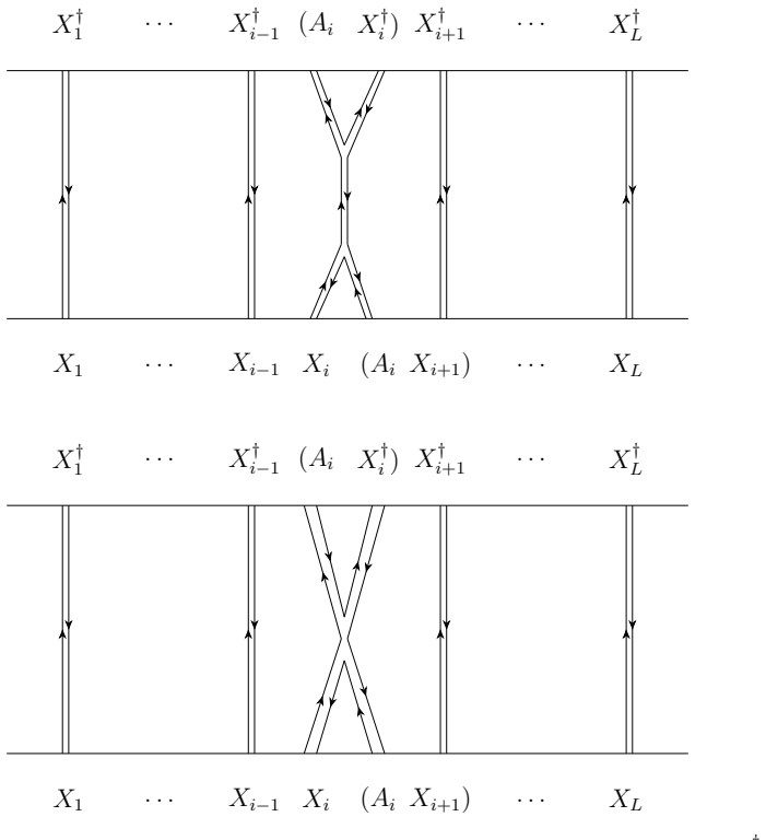
In these orbifold SCFTs the dilatation operator restricted to a chosen subsector is equivalent to a nearest-neighbor spin chain whose couplings are the marginal parameters; tuning the couplings drives the spectrum from Anderson localized to chaotic, as measured by standard spectral diagnostics.
What carries the argument
The effective nearest-neighbor spin-chain Hamiltonian whose interaction strengths are the marginal couplings of the SCFT and whose eigenvalues reproduce the anomalous dimensions in the subsector.
If this is right
- Chaotic statistics appear only when the marginal couplings are tuned away from generic values.
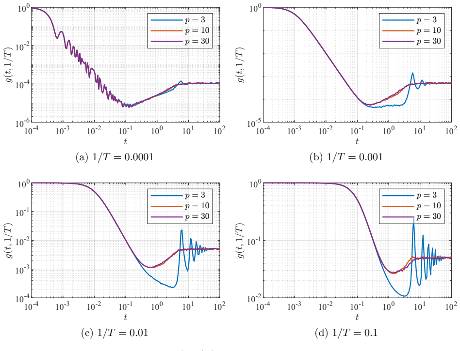
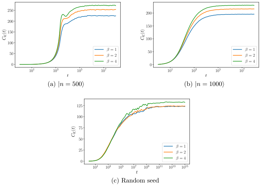
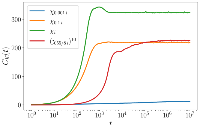
- Krylov complexity does not always register the same transition that level repulsion and the spectral form factor detect.
- The chaotic spectrum corresponds to a chaotic billiard in the target space of the string realization.
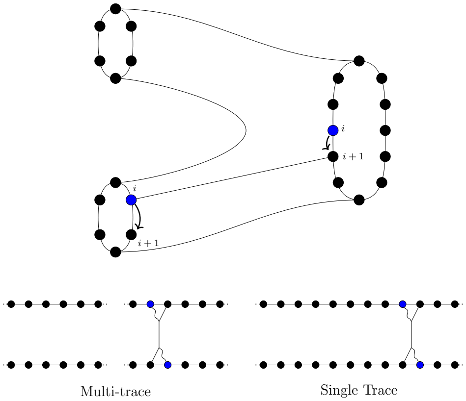
- At large N the holographic description must include multi-trace splitting and joining in addition to the single spin chain.
Where Pith is reading between the lines
- The spin-chain reduction may fail outside the chosen subsector once higher-order mixing terms become comparable.
- Analogous tuning of marginal parameters in other orbifold or quiver SCFTs could produce further controlled examples of chaotic spectra.
- The geometric billiard picture suggests that target-space curvature or flux choices could be adjusted to move the onset of chaos.
Load-bearing premise
The effective nearest-neighbor spin-chain Hamiltonian accurately captures the operator mixing in the chosen subsector for all values of the marginal couplings, without higher-order or non-local corrections that would alter the eigenvalue statistics.
What would settle it
An explicit computation of the full one-loop dilatation operator mixing matrix for a finite set of operators at a tuned marginal coupling that fails to exhibit level repulsion or spectral rigidity would falsify the claim that the spin-chain model controls the statistics.
Figures
read the original abstract
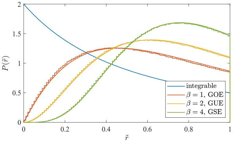
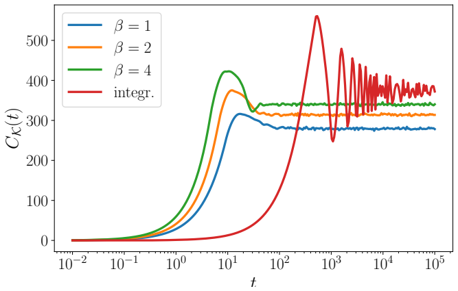
Chaotic dynamics play an important role in a number of physical systems. One of the qualitative hallmarks of this behavior is the appearance of a sufficiently "complex" spectrum of energy levels. This also makes it challenging to directly verify the onset of chaos in interacting quantum field theories. We present a class of 4D superconformal field theories (SCFTs) given by orbifolds of 4D $\mathcal{N} = 4$ Super Yang--Mills theory in which operator mixing in a controlled subsector is described by an effective spin chain in one spatial dimension with nearest neighbor interactions tuned by the marginal couplings of the SCFT. Tuning the marginal couplings results in a chaotic spectrum, while generically the spin chain exhibits Anderson localization. We diagnose the onset of chaos by analyzing the statistical distribution of eigenvalues of the dilatation operator, in particular properties such as eigenvalue level repulsion, spectral rigidity, and the spectral form factor. We also show that other diagnostics such as Krylov complexity sometimes do not faithfully capture this information. This structure defines a chaotic billiard in the target space of the stringy realization. We also comment on the large $N$ holographic dual description, where the controlled single spin chain approximation must be supplemented by multi-trace dynamics, i.e., the splitting and joining of multiple spin chains.
Editorial analysis
A structured set of objections, weighed in public.
Referee Report
Summary. The manuscript introduces a class of 4D orbifold SCFTs descending from N=4 SYM in which the one-loop dilatation operator, restricted to a protected subsector, reduces to a one-dimensional nearest-neighbor spin chain whose couplings are set by the marginal parameters of the SCFT. Tuning these parameters is claimed to drive a transition from Anderson localization to chaotic level statistics, diagnosed via eigenvalue repulsion, spectral rigidity, and the spectral form factor; generic values remain localized. The authors note that the large-N holographic description requires supplementing the single-chain picture with multi-trace splitting and joining, and they compare the diagnostics to Krylov complexity.
Significance. If the nearest-neighbor truncation remains valid for all values of the marginal couplings, the construction supplies a tunable, symmetry-protected example in which chaos versus localization can be studied directly in the spectrum of a 4D SCFT dilatation operator. This would be a concrete addition to the limited set of controlled QFT examples of quantum chaos and could inform holographic models of chaotic billiards. The explicit comparison of multiple spectral diagnostics is a positive feature.
major comments (3)
- [Abstract, §1] Abstract and §1: The central claim that the effective Hamiltonian remains exactly a tunable nearest-neighbor spin chain for arbitrary marginal couplings is stated without an explicit derivation or error estimate. The text acknowledges that the holographic dual requires multi-trace corrections, but does not demonstrate that the single-chain truncation itself acquires no non-local or higher-order mixing terms when the couplings are deformed away from the integrable locus. This assumption is load-bearing for the reported transition in level statistics.
- [§3] §3 (or equivalent section presenting the spin-chain Hamiltonian): No explicit check is supplied that the projection to the chosen subsector continues to eliminate longer-range interactions once the marginal couplings are varied. A concrete calculation for at least one representative value of the tuned couplings, including an estimate of the size of neglected terms, is required to support the chaos diagnostics.
- [§4] §4 (diagnostics section): The reported level-repulsion, rigidity, and spectral-form-factor results are presented as evidence of chaos, yet without a quantitative assessment of finite-size effects or of the range of couplings over which the nearest-neighbor approximation is controlled. The claim that these diagnostics are robust therefore rests on the unverified truncation.
minor comments (2)
- [§2] Notation for the marginal couplings and the precise definition of the subsector should be introduced earlier and used consistently.
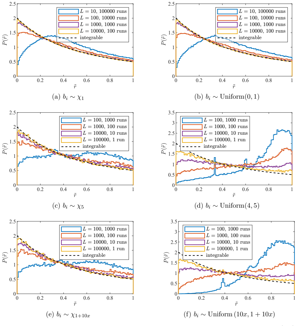
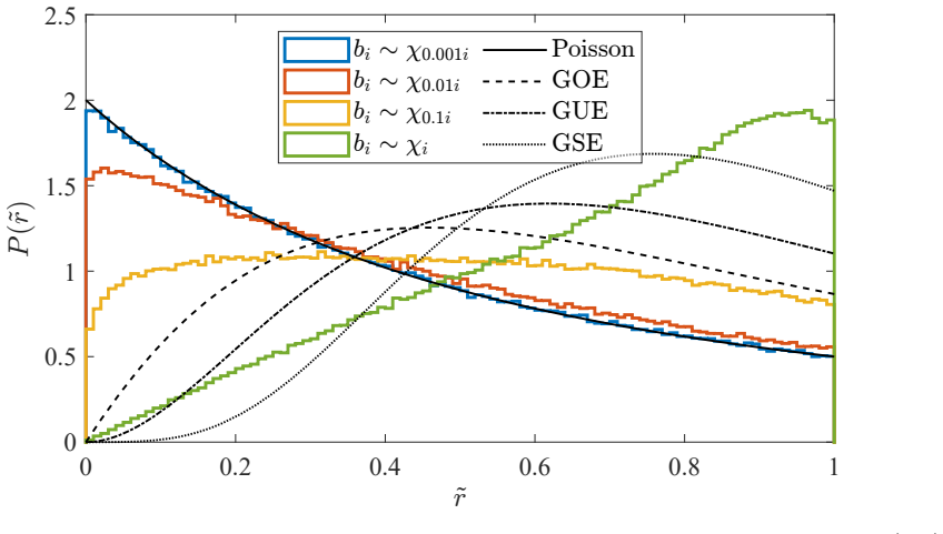
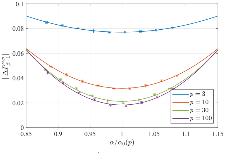
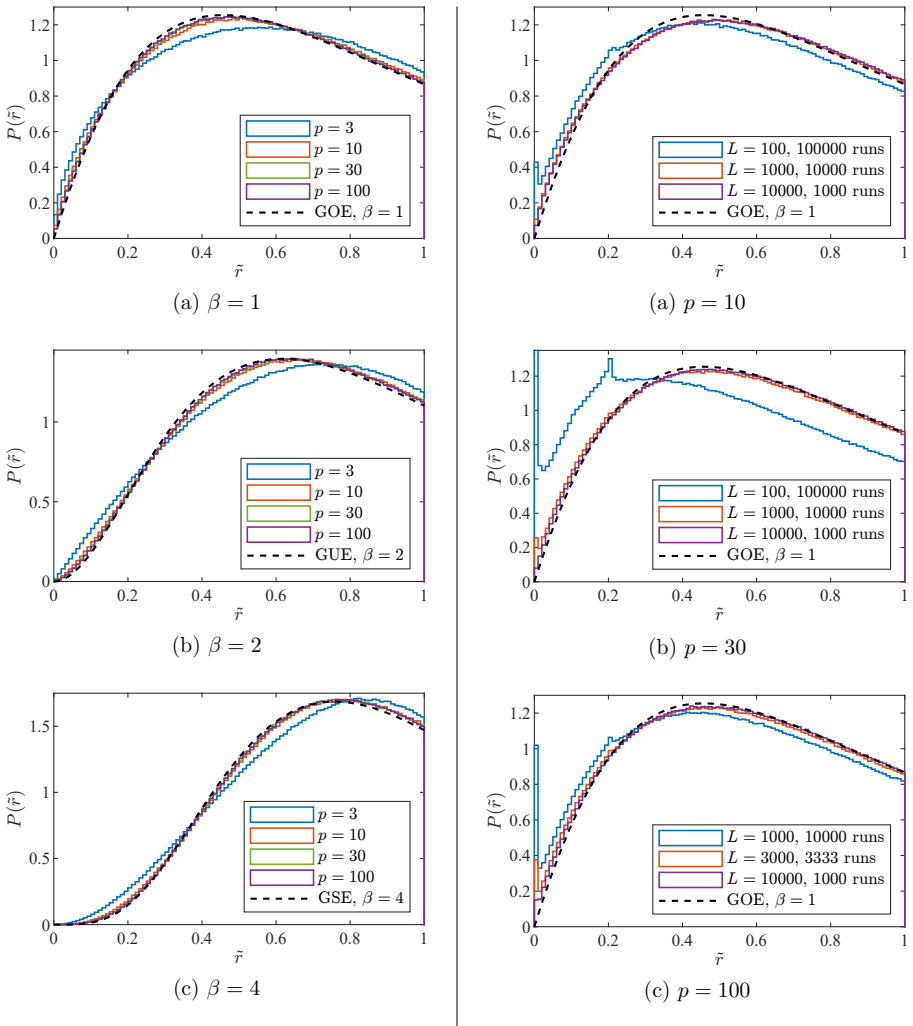
- [Figure 2] Figure captions for the spectral statistics plots should state the range of couplings and the system size used for each curve.
Simulated Author's Rebuttal
We thank the referee for the thorough review and for highlighting the need to strengthen the justification of the nearest-neighbor truncation. We address each major comment below and will incorporate the requested derivations, checks, and quantitative assessments into the revised manuscript.
read point-by-point responses
-
Referee: [Abstract, §1] Abstract and §1: The central claim that the effective Hamiltonian remains exactly a tunable nearest-neighbor spin chain for arbitrary marginal couplings is stated without an explicit derivation or error estimate. The text acknowledges that the holographic dual requires multi-trace corrections, but does not demonstrate that the single-chain truncation itself acquires no non-local or higher-order mixing terms when the couplings are deformed away from the integrable locus. This assumption is load-bearing for the reported transition in level statistics.
Authors: We agree that an explicit derivation was not provided in sufficient detail. In the revised manuscript we will expand the discussion in §2 with a complete one-loop calculation of the dilatation operator in the orbifold theory. This derivation shows that the orbifold projection together with the form of the superpotential terms continues to forbid non-nearest-neighbor mixing at one-loop order for arbitrary marginal couplings; any potential non-local contributions are shown to vanish identically within the protected subsector. An error estimate in the large-N limit will also be included. revision: yes
-
Referee: [§3] §3 (or equivalent section presenting the spin-chain Hamiltonian): No explicit check is supplied that the projection to the chosen subsector continues to eliminate longer-range interactions once the marginal couplings are varied. A concrete calculation for at least one representative value of the tuned couplings, including an estimate of the size of neglected terms, is required to support the chaos diagnostics.
Authors: We will add to §3 an explicit numerical check for a representative non-integrable value of the marginal couplings. The full mixing matrix within the subsector will be computed and compared against the nearest-neighbor truncation; the difference will be shown to be consistent with zero within the one-loop approximation, with an explicit bound on the size of any residual longer-range terms (suppressed by 1/N). revision: yes
-
Referee: [§4] §4 (diagnostics section): The reported level-repulsion, rigidity, and spectral-form-factor results are presented as evidence of chaos, yet without a quantitative assessment of finite-size effects or of the range of couplings over which the nearest-neighbor approximation is controlled. The claim that these diagnostics are robust therefore rests on the unverified truncation.
Authors: We accept that a quantitative assessment of finite-size effects and the validity range is needed. The revised §4 will present spectral statistics for multiple chain lengths (N=8 to N=20) to demonstrate convergence, together with a scan over the marginal-coupling plane that identifies the interval where the nearest-neighbor truncation reproduces the full subsector spectrum to within a specified tolerance. These additions will make the robustness of the chaos diagnostics explicit. revision: yes
Circularity Check
No significant circularity detected; derivation is self-contained.
full rationale
The paper defines an effective nearest-neighbor spin-chain Hamiltonian whose couplings are the external marginal parameters of the orbifold SCFT. Eigenvalue statistics (level repulsion, spectral rigidity, spectral form factor) are then computed directly from this Hamiltonian at different parameter values. This is a standard numerical or analytic evaluation of a parameterized matrix model, not a reduction of the claimed chaos to a fitted input or self-definition. No load-bearing self-citations, uniqueness theorems, or ansatze imported from prior author work are invoked to force the result. The central claim therefore remains independent of its inputs.
Axiom & Free-Parameter Ledger
free parameters (1)
- marginal couplings of the SCFT
axioms (2)
- domain assumption The orbifold preserves enough supersymmetry for the theory to remain conformal.
- domain assumption Operator mixing in the controlled subsector is captured by a nearest-neighbor spin-chain Hamiltonian.
Reference graph
Works this paper leans on
-
[1]
Statistical theory of the energy levels of complex systems. i,
F. J. Dyson, “Statistical theory of the energy levels of complex systems. i,”J. Math. Phys.3no. 1, (1962) 140–156
1962
-
[2]
Characterization of chaotic quantum spectra and universality of level fluctuation laws,
O. Bohigas, M. J. Giannoni, and C. Schmit, “Characterization of chaotic quantum spectra and universality of level fluctuation laws,”Phys. Rev. Lett.52(1984) 1–4
1984
-
[3]
Semiclassical foundation of universality in quantum chaos,
S. Muller, S. Heusler, P. Braun, F. Haake, and A. Altland, “Semiclassical foundation of universality in quantum chaos,”Phys. Rev. Lett.93(2004) 014103, arXiv:nlin/0401021
Pith/arXiv arXiv 2004
-
[4]
Random matrix theories in quantum physics: Common concepts,
T. Guhr, A. Muller-Groeling, and H. A. Weidenmuller, “Random matrix theories in quantum physics: Common concepts,”Phys. Rept.299(1998) 189–425, arXiv:cond-mat/9707301
Pith/arXiv arXiv 1998
-
[5]
Haake,Quantum Signatures of Chaos
F. Haake,Quantum Signatures of Chaos. Springer Series in Synergetics. Springer, Berlin, 2010
2010
-
[6]
Semiclassical theory of spectral rigidity,
M. V. Berry, “Semiclassical theory of spectral rigidity,”Proceedings of the Royal Society of London. A. Mathematical and Physical Sciences400no. 1819, (08, 1985) 229–251
1985
-
[7]
Quasiclassical Method in the Theory of Superconductivity,
A. I. Larkin and Y. N. Ovchinnikov, “Quasiclassical Method in the Theory of Superconductivity,”Soviet Journal of Experimental and Theoretical Physics28 (June, 1969) 1200
1969
-
[8]
Black Holes and the Butterfly Effect,
S. H. Shenker and D. Stanford, “Black Holes and the Butterfly Effect,”JHEP03 (2014) 067,arXiv:1306.0622 [hep-th]
Pith/arXiv arXiv 2014
-
[9]
J. Maldacena, S. H. Shenker, and D. Stanford, “A Bound on Chaos,”JHEP08 (2016) 106,arXiv:1503.01409 [hep-th]
Pith/arXiv arXiv 2016
-
[10]
Out-of-time-order correlators in quantum mechanics,
K. Hashimoto, K. Murata, and R. Yoshii, “Out-of-time-order correlators in quantum mechanics,”JHEP10(2017) 138,arXiv:1703.09435 [hep-th]
Pith/arXiv arXiv 2017
-
[11]
A Universal Operator Growth Hypothesis,
D. E. Parker, X. Cao, A. Avdoshkin, T. Scaffidi, and E. Altman, “A Universal Operator Growth Hypothesis,”Phys. Rev. X9no. 4, (2019) 041017, arXiv:1812.08657 [cond-mat.stat-mech]
arXiv 2019
-
[12]
On The Evolution Of Operator Complexity Beyond Scrambling,
J. L. F. Barb´ on, E. Rabinovici, R. Shir, and R. Sinha, “On The Evolution Of Operator Complexity Beyond Scrambling,”JHEP10(2019) 264,arXiv:1907.05393 [hep-th]
arXiv 2019
-
[13]
Euclidean operator growth and quantum chaos,
A. Avdoshkin and A. Dymarsky, “Euclidean operator growth and quantum chaos,” Phys. Rev. Res.2no. 4, (2020) 043234,arXiv:1911.09672 [cond-mat.stat-mech]. 58
arXiv 2020
-
[14]
Krylov complexity in conformal field theory,
A. Dymarsky and M. Smolkin, “Krylov complexity in conformal field theory,”Phys. Rev. D104no. 8, (2021) L081702,arXiv:2104.09514 [hep-th]
arXiv 2021
-
[15]
Geometry of Krylov complexity,
P. Caputa, J. M. Magan, and D. Patramanis, “Geometry of Krylov complexity,” Phys. Rev. Res.4no. 1, (2022) 013041,arXiv:2109.03824 [hep-th]
arXiv 2022
-
[16]
Quantum chaos and the complexity of spread of states,
V. Balasubramanian, P. Caputa, J. M. Magan, and Q. Wu, “Quantum chaos and the complexity of spread of states,”Phys. Rev. D106no. 4, (2022) 046007, arXiv:2202.06957 [hep-th]
arXiv 2022
-
[17]
Quantum complexity in gravity, quantum field theory, and quantum information science,
S. Baiguera, V. Balasubramanian, P. Caputa, S. Chapman, J. Haferkamp, M. P. Heller, and N. Y. Halpern, “Quantum complexity in gravity, quantum field theory, and quantum information science,”Phys. Rept.1159(2026) 1–77, arXiv:2503.10753 [hep-th]
arXiv 2026
-
[18]
Quantum dynamics in Krylov space: Methods and applications,
P. Nandy, A. S. Matsoukas-Roubeas, P. Mart´ ınez-Azcona, A. Dymarsky, and A. del Campo, “Quantum dynamics in Krylov space: Methods and applications,”Phys. Rept.1125-1128(2025) 1–82,arXiv:2405.09628 [quant-ph]
Pith/arXiv arXiv 2025
-
[19]
Operator complexity: a journey to the edge of Krylov space,
E. Rabinovici, A. S´ anchez-Garrido, R. Shir, and J. Sonner, “Operator complexity: a journey to the edge of Krylov space,”JHEP06(2021) 062,arXiv:2009.01862 [hep-th]
arXiv 2021
-
[20]
Krylov localization and suppression of complexity,
E. Rabinovici, A. S´ anchez-Garrido, R. Shir, and J. Sonner, “Krylov localization and suppression of complexity,”JHEP03(2022) 211,arXiv:2112.12128 [hep-th]
arXiv 2022
-
[21]
Krylov complexity from integrability to chaos,
E. Rabinovici, A. S´ anchez-Garrido, R. Shir, and J. Sonner, “Krylov complexity from integrability to chaos,”JHEP07(2022) 151,arXiv:2207.07701 [hep-th]
arXiv 2022
-
[22]
Tridiagonalizing random matrices,
V. Balasubramanian, J. M. Magan, and Q. Wu, “Tridiagonalizing random matrices,” Phys. Rev. D107no. 12, (2023) 126001,arXiv:2208.08452 [hep-th]
arXiv 2023
-
[23]
Krylov complexity in quantum field theory, and beyond,
A. Avdoshkin, A. Dymarsky, and M. Smolkin, “Krylov complexity in quantum field theory, and beyond,”JHEP06(2024) 066,arXiv:2212.14429 [hep-th]
arXiv 2024
-
[24]
Quantum chaos, integrability, and late times in the Krylov basis,
V. Balasubramanian, J. M. Magan, and Q. Wu, “Quantum chaos, integrability, and late times in the Krylov basis,”Phys. Rev. E111no. 1, (2025) 014218, arXiv:2312.03848 [hep-th]
arXiv 2025
-
[25]
Chaos and integrability in triangular billiards,
V. Balasubramanian, R. N. Das, J. Erdmenger, and Z.-Y. Xian, “Chaos and integrability in triangular billiards,”J. Stat. Mech.2025no. 3, (2025) 033202, arXiv:2407.11114 [hep-th]
arXiv 2025
-
[26]
Variations on a Theme of Krylov,
V. Balasubramanian, P. Caputa, and J. Sim´ on, “Variations on a Theme of Krylov,” arXiv:2511.03775 [hep-th]. 59
-
[27]
E. Rabinovici, A. S´ anchez-Garrido, R. Shir, and J. Sonner, “Krylov Complexity,” arXiv:2507.06286 [hep-th]
-
[28]
On the CFT Operator Spectrum at Large Global Charge,
S. Hellerman, D. Orlando, S. Reffert, and M. Watanabe, “On the CFT Operator Spectrum at Large Global Charge,”JHEP12(2015) 071,arXiv:1505.01537 [hep-th]
arXiv 2015
-
[29]
Selected topics in the large quantum number expansion,
L. ´A. Gaum´ e, D. Orlando, and S. Reffert, “Selected topics in the large quantum number expansion,”Phys. Rept.933(2021) 1–66,arXiv:2008.03308 [hep-th]
arXiv 2021
-
[30]
Strings in flat space and pp waves fromN= 4 Super Yang Mills,
D. E. Berenstein, J. M. Maldacena, and H. S. Nastase, “Strings in flat space and pp waves fromN= 4 Super Yang Mills,”JHEP04(2002) 013,arXiv:hep-th/0202021
Pith/arXiv arXiv 2002
-
[31]
Chaotic spin chains in AdS/CFT,
T. McLoughlin and A. Spiering, “Chaotic spin chains in AdS/CFT,”JHEP09 (2022) 240,arXiv:2202.12075 [hep-th]
arXiv 2022
-
[32]
D-branes, quivers, and ALE instantons,
M. R. Douglas and G. W. Moore, “D-branes, quivers, and ALE instantons,” arXiv:hep-th/9603167
-
[33]
4d Conformal Theories and Strings on Orbifolds,
S. Kachru and E. Silverstein, “4d Conformal Theories and Strings on Orbifolds,” Phys. Rev. Lett.80(1998) 4855–4858,arXiv:hep-th/9802183
Pith/arXiv arXiv 1998
-
[34]
On conformal field theories in four-dimensions,
A. E. Lawrence, N. Nekrasov, and C. Vafa, “On conformal field theories in four-dimensions,”Nucl. Phys. B533(1998) 199–209,arXiv:hep-th/9803015
Pith/arXiv arXiv 1998
-
[35]
The Bethe Ansatz forZ S Orbifolds ofN= 4 Super Yang-Mills Theory,
N. Beisert and R. Roiban, “The Bethe Ansatz forZ S Orbifolds ofN= 4 Super Yang-Mills Theory,”JHEP11(2005) 037,arXiv:hep-th/0510209
Pith/arXiv arXiv 2005
-
[36]
Exactly marginal deformations of quiver gauge theories as seen from brane tilings,
Y. Imamura, H. Isono, K. Kimura, and M. Yamazaki, “Exactly marginal deformations of quiver gauge theories as seen from brane tilings,”Prog. Theor. Phys. 117(2007) 923–955,arXiv:hep-th/0702049
Pith/arXiv arXiv 2007
-
[37]
Matrix models for beta ensembles,
I. Dumitriu and A. Edelman, “Matrix models for beta ensembles,”J. Math. Phys.43 no. 11, (2002) 5830–5847,arXiv:math-ph/0206043
Pith/arXiv arXiv 2002
-
[38]
Absence of Diffusion in Certain Random Lattices,
P. W. Anderson, “Absence of Diffusion in Certain Random Lattices,”Phys. Rev.109 (1958) 1492–1505
1958
-
[39]
Statistical theory of the energy levels of complex systems. ii,
F. J. Dyson, “Statistical theory of the energy levels of complex systems. ii,”J. Math. Phys.3no. 1, (1962) 157–165
1962
-
[40]
Statistical theory of the energy levels of complex systems. iii,
F. J. Dyson, “Statistical theory of the energy levels of complex systems. iii,”J. Math. Phys.3no. 1, (1962) 166–175
1962
-
[41]
Statistical theory of the energy levels of complex systems. iv,
F. J. Dyson and M. L. Mehta, “Statistical theory of the energy levels of complex systems. iv,”J. Math. Phys.4no. 5, (1963) 701–712. 60
1963
-
[42]
Black Holes and Random Matrices,
J. S. Cotler, G. Gur-Ari, M. Hanada, J. Polchinski, P. Saad, S. H. Shenker, D. Stanford, A. Streicher, and M. Tezuka, “Black Holes and Random Matrices,” JHEP05(2017) 118,arXiv:1611.04650 [hep-th]. [Erratum: JHEP 09, 002 (2018)]
Pith/arXiv arXiv 2017
-
[43]
Random matrix theory for complexity growth and black hole interiors,
A. Kar, L. Lamprou, M. Rozali, and J. Sully, “Random matrix theory for complexity growth and black hole interiors,”JHEP01(2022) 016,arXiv:2106.02046 [hep-th]
arXiv 2022
-
[44]
Krylov Complexity in Quantum Field Theory,
K. Adhikari, S. Choudhury, and A. Roy, “Krylov Complexity in Quantum Field Theory,”Nucl. Phys. B993(2023) 116263,arXiv:2204.02250 [hep-th]
arXiv 2023
-
[45]
Krylov complexity in open quantum systems,
C. Liu, H. Tang, and H. Zhai, “Krylov complexity in open quantum systems,”Phys. Rev. Res.5no. 3, (2023) 033085,arXiv:2207.13603 [cond-mat.str-el]
arXiv 2023
-
[46]
Krylov complexity in large q and double-scaled SYK model,
B. Bhattacharjee, P. Nandy, and T. Pathak, “Krylov complexity in large q and double-scaled SYK model,”JHEP08(2023) 099,arXiv:2210.02474 [hep-th]
arXiv 2023
-
[47]
Krylov complexity in Calabi–Yau quantum mechanics,
B.-n. Du and M.-x. Huang, “Krylov complexity in Calabi–Yau quantum mechanics,” Int. J. Mod. Phys. A38no. 22n23, (2023) 2350126,arXiv:2212.02926 [hep-th]
arXiv 2023
-
[48]
Assessing the saturation of Krylov complexity as a measure of chaos,
B. L. Espa˜ nol and D. A. Wisniacki, “Assessing the saturation of Krylov complexity as a measure of chaos,”Phys. Rev. E107no. 2, (2023) 024217,arXiv:2212.06619 [quant-ph]
arXiv 2023
-
[49]
Krylov complexity in free and interacting scalar field theories with bounded power spectrum,
H. A. Camargo, V. Jahnke, K.-Y. Kim, and M. Nishida, “Krylov complexity in free and interacting scalar field theories with bounded power spectrum,”JHEP05(2023) 226,arXiv:2212.14702 [hep-th]
arXiv 2023
-
[50]
On Krylov complexity in open systems: an approach via bi-Lanczos algorithm,
A. Bhattacharya, P. Nandy, P. P. Nath, and H. Sahu, “On Krylov complexity in open systems: an approach via bi-Lanczos algorithm,”JHEP12(2023) 066, arXiv:2303.04175 [quant-ph]
arXiv 2023
-
[51]
Krylov complexity and chaos in quantum mechanics,
K. Hashimoto, K. Murata, N. Tanahashi, and R. Watanabe, “Krylov complexity and chaos in quantum mechanics,”JHEP11(2023) 040,arXiv:2305.16669 [hep-th]
arXiv 2023
-
[52]
Krylov complexity of density matrix operators,
P. Caputa, H.-S. Jeong, S. Liu, J. F. Pedraza, and L.-C. Qu, “Krylov complexity of density matrix operators,”JHEP05(2024) 337,arXiv:2402.09522 [hep-th]
arXiv 2024
-
[53]
Krylov complexity of deformed conformal field theories,
A. Chattopadhyay, V. Malvimat, and A. Mitra, “Krylov complexity of deformed conformal field theories,”JHEP08(2024) 053,arXiv:2405.03630 [hep-th]
arXiv 2024
-
[54]
Krylov complexity as an order parameter for quantum chaotic-integrable transitions,
M. Baggioli, K.-B. Huh, H.-S. Jeong, K.-Y. Kim, and J. F. Pedraza, “Krylov complexity as an order parameter for quantum chaotic-integrable transitions,”Phys. Rev. Res.7no. 2, (2025) 023028,arXiv:2407.17054 [hep-th]. 61
arXiv 2025
-
[55]
Krylov complexity as a probe for chaos,
M. Alishahiha, S. Banerjee, and M. J. Vasli, “Krylov complexity as a probe for chaos,”Eur. Phys. J. C85no. 7, (2025) 749,arXiv:2408.10194 [hep-th]
arXiv 2025
-
[56]
B. Craps, O. Evnin, and G. Pascuzzi, “Multiseed Krylov Complexity,”Phys. Rev. Lett.134no. 5, (2025) 050402,arXiv:2409.15666 [quant-ph]
arXiv 2025
-
[57]
Spread complexity for the planar limit of holography,
R. N. Das, S. Demulder, J. Erdmenger, and C. Northe, “Spread complexity for the planar limit of holography,”JHEP06(2025) 166,arXiv:2412.09673 [hep-th]
arXiv 2025
-
[58]
Dependence of Krylov complexity saturation on the initial operator and state,
S. PG, J. B. Kannan, R. Modak, and S. Aravinda, “Dependence of Krylov complexity saturation on the initial operator and state,”Phys. Rev. E112no. 3, (2025) L032203,arXiv:2503.03400 [quant-ph]
arXiv 2025
-
[59]
Krylov exponents and power spectra for maximal quantum chaos: an EFT approach,
S. Demulder, M. Knysh, and A. Rolph, “Krylov exponents and power spectra for maximal quantum chaos: an EFT approach,”JHEP04(2026) 059, arXiv:2508.05444 [hep-th]
arXiv 2026
-
[60]
Anderson localization: A view from Krylov space,
J. C. Peacock, V. Oganesyan, and D. Sels, “Anderson localization: A view from Krylov space,”Phys. Rev. B113no. 6, (2026) 064204,arXiv:2510.26920 [cond-mat.dis-nn]
arXiv 2026
-
[61]
Krylov Dynamics and Operator Growth in Time-Dependent Systems via Lie Algebras,
A. Grabarits, E. Medina-Guerra, and A. del Campo, “Krylov Dynamics and Operator Growth in Time-Dependent Systems via Lie Algebras,”arXiv:2605.05290 [quant-ph]
-
[62]
Towards a Refinement of Krylov Complexity: Scrambling, Classical Operator Growth and Replicas,
H. A. Camargo, Y. Fu, K.-Y. Kim, and Y. H. Park, “Towards a Refinement of Krylov Complexity: Scrambling, Classical Operator Growth and Replicas,” arXiv:2603.19359 [hep-th]
-
[63]
Krylov Complexity in Supersymmetric Large-N Quantum Mechanics,
E. Alfinito and M. Beccaria, “Krylov Complexity in Supersymmetric Large-N Quantum Mechanics,”arXiv:2603.16291 [hep-th]
-
[64]
Krylov state complexity for BMN matrix model,
D. Roychowdhury, “Krylov state complexity for BMN matrix model,” arXiv:2605.10786 [hep-th]
-
[65]
Krylov Complexity for Plane Wave Matrix Model,
D. Roychowdhury, “Krylov Complexity for Plane Wave Matrix Model,” arXiv:2605.26055 [hep-th]
-
[66]
Holographic Krylov Complexity for Charged, Composite and Extended Probes,
H. Nastase, C. Nunez, and D. Roychowdhury, “Holographic Krylov Complexity for Charged, Composite and Extended Probes,”arXiv:2604.07432 [hep-th]
-
[67]
Holographic Krylov complexity inN= 4 SYM,
A. Fatemiabhari, H. Nastase, and D. Roychowdhury, “Holographic Krylov complexity inN= 4 SYM,”arXiv:2511.19286 [hep-th]
-
[68]
Krylov-space anatomy and spread complexity of a disordered quantum spin chain,
B. Pain, D. E. Logan, and S. Roy, “Krylov-space anatomy and spread complexity of a disordered quantum spin chain,”arXiv:2603.25724 [cond-mat.dis-nn]. 62
-
[69]
Holographic Krylov complexity in confining gauge theories,
A. Fatemiabhari, H. Nastase, C. Nunez, and D. Roychowdhury, “Holographic Krylov complexity in confining gauge theories,”arXiv:2511.22717 [hep-th]
-
[70]
Holographic Krylov Complexity for Conformal Quiver Gauge Theories,
A. Fatemiabhari, H. Nastase, C. Nunez, and D. Roychowdhury, “Holographic Krylov Complexity for Conformal Quiver Gauge Theories,”arXiv:2512.14812 [hep-th]
-
[71]
Complexity and Operator Growth in Holographic 6d SCFTs,
A. Fatemiabhari, C. Nunez, and R. T. Santamaria, “Complexity and Operator Growth in Holographic 6d SCFTs,”arXiv:2603.10106 [hep-th]
-
[72]
Krylov Complexity, Confinement and Universality,
A. Fatemiabhari and C. Nunez, “Krylov Complexity, Confinement and Universality,” arXiv:2602.17757 [hep-th]
-
[73]
Probing Weak Chaos inN= 4 Super Yang-Mills and Long-Range Spin Chains,
P. Caputa, B. Creed, R. N. Das, S. Demulder, and T. McLoughlin, “Probing Weak Chaos inN= 4 Super Yang-Mills and Long-Range Spin Chains,”arXiv:2606.18351 [hep-th]
-
[74]
Sachdev-Ye-Kitaev model and thermalization on the boundary of many-body localized fermionic symmetry-protected topological states,
Y.-Z. You, A. W. W. Ludwig, and C. Xu, “Sachdev-Ye-Kitaev model and thermalization on the boundary of many-body localized fermionic symmetry-protected topological states,”Physical Review B95no. 11, (Mar., 2017) 115150
2017
-
[75]
Spectral and thermodynamic properties of the Sachdev-Ye-Kitaev model,
A. M. Garc´ ıa-Garc´ ıa and J. J. M. Verbaarschot, “Spectral and thermodynamic properties of the Sachdev-Ye-Kitaev model,”Phys. Rev. D94no. 12, (2016) 126010, arXiv:1610.03816 [hep-th]
Pith/arXiv arXiv 2016
-
[76]
Y. Chen, H. W. Lin, and S. H. Shenker, “BPS chaos,”SciPost Phys.18no. 2, (2025) 072,arXiv:2407.19387 [hep-th]
Pith/arXiv arXiv 2025
-
[77]
Localization of interacting fermions at high temperature,
V. Oganesyan and D. A. Huse, “Localization of interacting fermions at high temperature,”Phys. Rev. B75no. 15, (2007) 155111
2007
-
[78]
Distribution of the Ratio of Consecutive Level Spacings in Random Matrix Ensembles,
Y. Y. Atas, E. Bogomolny, O. Giraud, and G. Roux, “Distribution of the Ratio of Consecutive Level Spacings in Random Matrix Ensembles,”Phys. Rev. Lett.110 no. 8, (2013) 084101
2013
-
[79]
An iteration method for the solution of the eigenvalue problem of linear differential and integral operators,
C. Lanczos, “An iteration method for the solution of the eigenvalue problem of linear differential and integral operators,”J. Res. Natl. Bur. Stand. B45(1950) 255–282
1950
-
[80]
Akemann, J
G. Akemann, J. Baik, and P. Di Francesco,The Oxford Handbook of Random Matrix Theory. Oxford Handbooks in Mathematics. Oxford University Press, 9, 2011
2011
discussion (0)
Sign in with ORCID, Apple, or X to comment. Anyone can read and Pith papers without signing in.