Analytical and fitting formulae for solutions to Lyman-alpha radiative transfer equations: the effects of geometry, recoil, and velocity gradients
Pith reviewed 2026-06-29 02:10 UTC · model grok-4.3
The pith
Analytical formulae and fitting tools solve Lyman-alpha transfer under geometry, recoil, and velocity gradients
A machine-rendered reading of the paper's core claim, the machinery that carries it, and where it could break.
Core claim
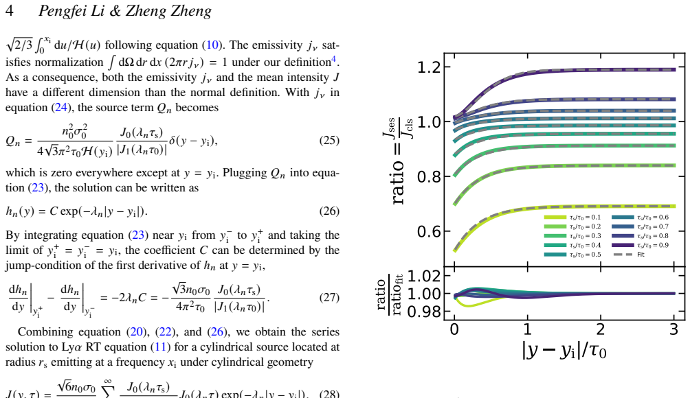
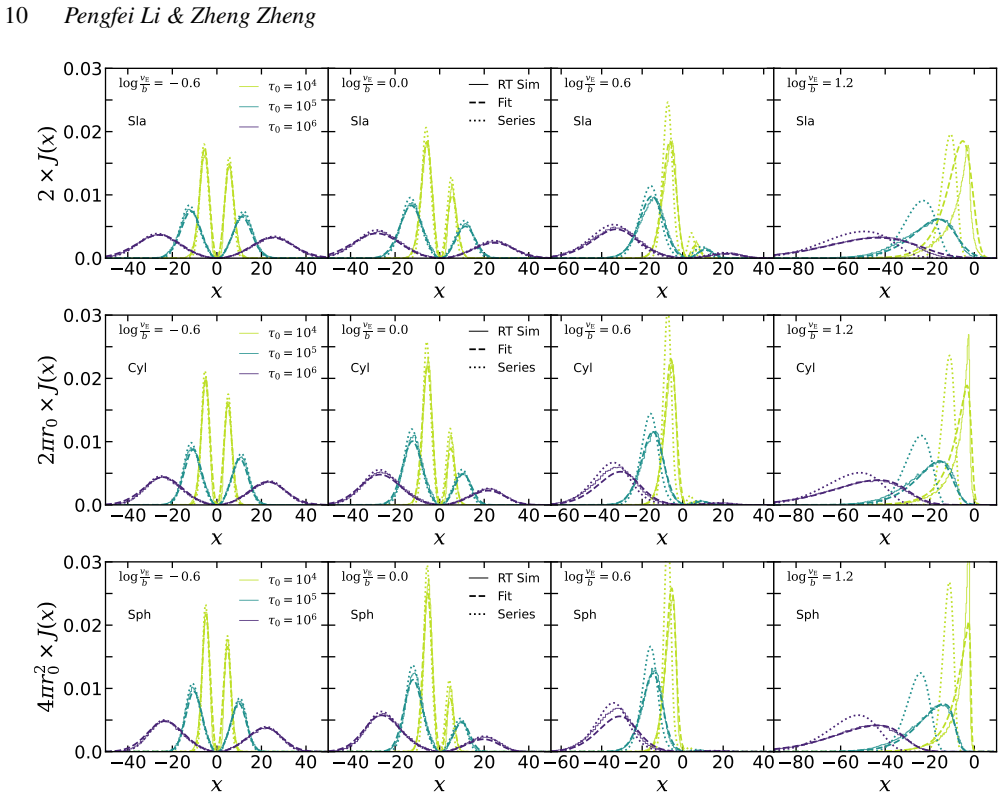
The paper establishes analytical formulae for Lyα spectra in cylindrical geometry, verifies them with Monte Carlo simulations, and provides series solutions for velocity gradients that agree well for small values of v_E/b but require empirical extension for large values up to 100, resulting in fitting formulae that match simulations at large optical depths. The work completes the set of solutions under simple geometries and supplies practical analytical expressions incorporating recoil and bulk motion.
What carries the argument
Series solutions to the Lyα RT equations with constant velocity gradients, combined with empirically extended functional forms fitted to Monte Carlo simulation results for large gradients.
If this is right
- The fitting formulae enable accurate modeling of Lyα line profiles in galaxies with strong outflows or inflows without running full simulations.
- Completion of analytical solutions across cylindrical, slab, and spherical geometries allows systematic study of how cloud shape affects emergent Lyα spectra.
- The empirical recoil modification supplies a practical method to include frequency shifts from atomic recoil in analytical studies of resonant line transfer.
- For velocity gradients comparable to the thermal velocity, the series solutions can be used directly in theoretical calculations of photon escape.
Where Pith is reading between the lines
- These analytical expressions could be incorporated into semi-analytic galaxy models to predict Lyα emission and absorption profiles more efficiently across large parameter spaces.
- The principle of extending functional forms to match simulations at extreme gradients may generalize to other resonant scattering problems with bulk velocity fields.
- Comparison of the formulae against integral-field observations of high-redshift Lyα emitters could provide an external check on accuracy at the largest velocity gradients.
Load-bearing premise
The empirical modifications to recoil-free spectra and the extended functional forms for large velocity gradients remain accurate when applied outside the specific parameters of the Monte Carlo simulations used to constrain them.
What would settle it
New Monte Carlo radiative transfer simulations at v_E/b values of 50 and 200 with optical depths around 10^5 to 10^6, followed by direct comparison of the predicted spectra to the fitting formulae, would test whether the claimed improvement holds.
Figures
read the original abstract
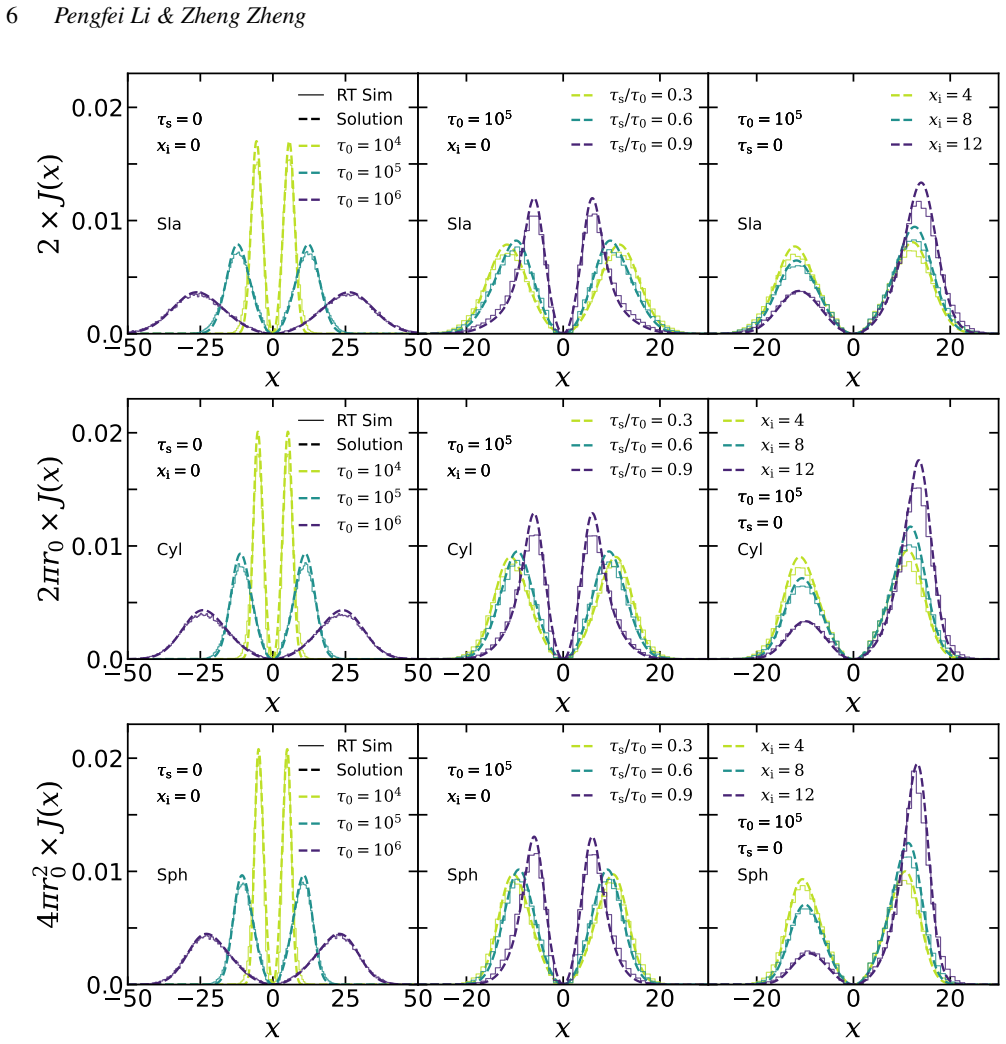
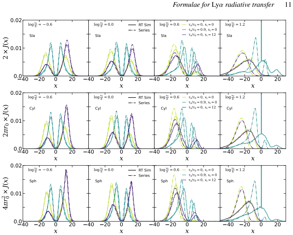
Lyman-alpha (Ly$\alpha$) radiative transfer (RT) is important in many astrophysical environments and governed by multiple physical processes. In this paper, we provide analytical formulae/procedures for the solutions to Ly$\alpha$ RT equations under three simple geometrical symmetries and investigate the effects of atomic recoil and gas bulk motion. We first study Ly$\alpha$ spectra by solving Ly$\alpha$ RT equations for a static, uniform gas cloud under cylindrical geometry. The solution is verified through Ly$\alpha$ Monte Carlo RT simulations, and compared to those under slab and spherical geometries in literature. Second, to characterise the recoil effect, we empirically modify recoil-free Ly$\alpha$ spectra. The method is motivated by Ly$\alpha$ RT equations with recoil and justified by simulations. Finally, we account for constant velocity gradients in Ly$\alpha$ RT equations and obtain series solutions for Ly$\alpha$ spectra. The solutions demonstrate good agreement to Ly$\alpha$ spectra from simulations for small velocity gradients (i.e. edge velocity $v_{\rm E}$ of a cloud being comparable to the thermal velocity $b$) but become less accurate for large ones. To characterise Ly$\alpha$ spectra under large velocity gradients, we empirically extend the functional form of solutions and constrain them from fitting simulated Ly$\alpha$ spectra. The resulting fitting formulae show significant improvement for large velocity gradients ($v_{\rm E}/b \sim 100$) under large optical depths. The analytical study of Ly$\alpha$ spectra in this work completes the set of solutions under simple geometries, provides physical insights for Ly$\alpha$ RT under recoil and velocity gradient, and develops analytical tools for theoretical studies that require inputs from Ly$\alpha$ RT.
Editorial analysis
A structured set of objections, weighed in public.
Referee Report
Summary. The paper derives analytical solutions to the Lyα radiative transfer equations for a static uniform gas cloud in cylindrical geometry (verified against Monte Carlo simulations and compared to slab/spherical cases), introduces an empirical modification to recoil-free spectra motivated by the recoil-inclusive equations but justified by simulations, and obtains series solutions for constant velocity gradients that agree with simulations at small v_E/b but are empirically extended in functional form and constrained by fitting to simulated spectra for large gradients (v_E/b ~100) at high optical depths. It claims these complete the set of solutions under simple geometries and supply practical analytical/fitting tools.
Significance. If the results hold, the static cylindrical solutions (cross-checked with Monte Carlo RT simulations) add a useful independent geometry to the existing slab and spherical literature, while the recoil modification and velocity-gradient fitting formulae could serve as efficient inputs for theoretical modeling of Lyα spectra in astrophysical environments with bulk motions. The explicit verification of the static case against simulations is a concrete strength supporting reproducibility.
major comments (2)
- [Velocity-gradient section] Velocity-gradient section (abstract and corresponding derivation): the series solutions from the RT equations are stated to become less accurate at large v_E/b; the empirically extended functional form is then 'constrained from fitting simulated Lyα spectra' with no mention of cross-validation on independent runs or error estimates independent of the fitting data. This is load-bearing for the central claim of 'significant improvement' at v_E/b ~100 under large optical depths, as accuracy is secured only by agreement with the same class of Monte Carlo runs used to fit the parameters.
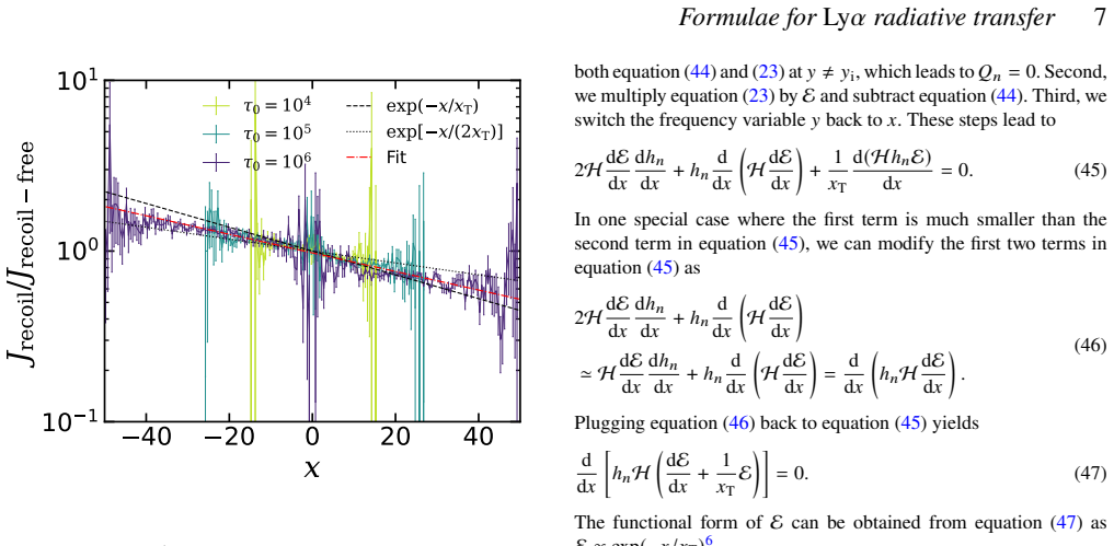
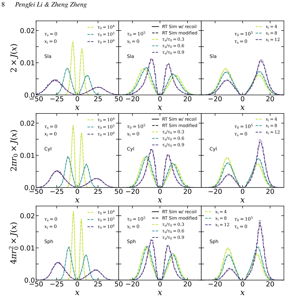
- [Recoil-effect section] Recoil-effect section (abstract): the empirical modification of recoil-free spectra is described as 'motivated by' the RT equations with recoil but 'justified by simulations.' Because the modification is not derived from the full recoil-inclusive equations, the claim that the work 'provides physical insights for Lyα RT under recoil' rests on post-hoc agreement rather than an independent derivation or quantitative test of the modification's fidelity beyond the fitting simulations.
minor comments (2)
- The abstract refers to 'the resulting fitting formulae' and 'analytical study' but does not indicate whether the explicit functional forms, fitting coefficients, or step-by-step procedures are provided in sufficient detail for direct implementation by readers.
- Notation for velocity gradient (v_E/b) and optical depth should be defined at first use with reference to the relevant equation to aid clarity for readers comparing to prior slab/spherical work.
Simulated Author's Rebuttal
We thank the referee for the careful review and constructive feedback on our manuscript. We address each major comment below and outline the revisions we will make.
read point-by-point responses
-
Referee: [Velocity-gradient section] Velocity-gradient section (abstract and corresponding derivation): the series solutions from the RT equations are stated to become less accurate at large v_E/b; the empirically extended functional form is then 'constrained from fitting simulated Lyα spectra' with no mention of cross-validation on independent runs or error estimates independent of the fitting data. This is load-bearing for the central claim of 'significant improvement' at v_E/b ~100 under large optical depths, as accuracy is secured only by agreement with the same class of Monte Carlo runs used to fit the parameters.
Authors: We agree that the manuscript does not describe cross-validation on independent simulation runs or report error estimates separate from the fitting data. This is a valid concern for the robustness of the large-gradient fitting formulae. In the revised version we will (i) generate an independent set of Monte Carlo runs, (ii) perform cross-validation, and (iii) include quantitative error metrics (e.g., mean fractional deviation and maximum deviation) evaluated on the held-out data. These additions will be reported in the velocity-gradient section and the abstract will be updated accordingly. revision: yes
-
Referee: [Recoil-effect section] Recoil-effect section (abstract): the empirical modification of recoil-free spectra is described as 'motivated by' the RT equations with recoil but 'justified by simulations.' Because the modification is not derived from the full recoil-inclusive equations, the claim that the work 'provides physical insights for Lyα RT under recoil' rests on post-hoc agreement rather than an independent derivation or quantitative test of the modification's fidelity beyond the fitting simulations.
Authors: The modification is indeed empirical; it is not obtained by solving the full recoil-inclusive equations analytically. Its functional form is chosen to reproduce the leading-order effect suggested by those equations and is then calibrated to simulations. We will revise the abstract and the relevant section to state more explicitly that the approach is empirical, that the physical motivation is limited to the choice of functional form, and that the quantitative support comes from simulation agreement. The claim of “physical insights” will be qualified to reflect this scope. revision: partial
Circularity Check
Empirical recoil modification and velocity-gradient extensions are constrained by fitting to Monte Carlo simulations
specific steps
-
fitted input called prediction
[Abstract]
"Second, to characterise the recoil effect, we empirically modify recoil-free Lyα spectra. The method is motivated by Lyα RT equations with recoil and justified by simulations."
The modification is not obtained by solving the RT equations with recoil; it is an empirical adjustment whose validity rests on agreement with Monte Carlo outputs rather than independent derivation.
-
fitted input called prediction
[Abstract]
"To characterise Lyα spectra under large velocity gradients, we empirically extend the functional form of solutions and constrain them from fitting simulated Lyα spectra. The resulting fitting formulae show significant improvement for large velocity gradients (v_E/b ∼ 100) under large optical depths."
The extended functional form is obtained by fitting parameters to the same class of Monte Carlo spectra; the reported improvement at large gradients is therefore a direct consequence of the fitting procedure rather than an independent prediction from the RT equations.
full rationale
Static cylindrical solutions are derived from the RT equations and verified by simulation. However, the recoil characterisation uses an empirical modification 'justified by simulations' rather than derived from the equations with recoil. For large velocity gradients, series solutions from the equations are extended by an empirical functional form whose parameters are 'constrain[ed] from fitting simulated Lyα spectra', so the claimed improvement at v_E/b ~100 is secured by agreement with the same simulations used to fit the parameters. This matches the 'fitted_input_called_prediction' pattern for the two key extensions that complete the claimed solution set. No self-citation chains or self-definitional reductions appear in the provided text.
Axiom & Free-Parameter Ledger
free parameters (1)
- parameters in empirical recoil modification and large-gradient fitting form
axioms (1)
- domain assumption Uniform density and temperature within the cloud; constant velocity gradient; complete frequency redistribution in the absence of recoil
Reference graph
Works this paper leans on
-
[1]
P Cygni type Ly from starburst galaxies. , keywords =. doi:10.1046/j.1365-8711.2003.06353.x , archivePrefix =. astro-ph/0204004 , primaryClass =
-
[2]
The MUSE 3D view of the Hubble Deep Field South
The MUSE 3D view of the Hubble Deep Field South. , keywords =. doi:10.1051/0004-6361/201425419 , archivePrefix =. 1411.7667 , primaryClass =
work page internal anchor Pith review Pith/arXiv arXiv doi:10.1051/0004-6361/201425419
-
[3]
The MUSE Extremely Deep Field: The cosmic web in emission at high redshift. , keywords =. doi:10.1051/0004-6361/202039887 , archivePrefix =. 2102.05516 , primaryClass =
-
[4]
The MUSE Hubble Ultra Deep Field surveys: Data release II. , keywords =. doi:10.1051/0004-6361/202244187 , archivePrefix =. 2211.08493 , primaryClass =
-
[5]
A model for infall around virialized haloes. , keywords =. doi:10.1111/j.1365-2966.2004.07177.x , archivePrefix =. astro-ph/0212458 , primaryClass =
-
[6]
Faint extended Ly emission due to star formation at the centre of high column density QSO absorption systems. , keywords =. doi:10.1111/j.1365-2966.2009.16172.x , archivePrefix =. 0912.1345 , primaryClass =
-
[7]
Beamed Lyman Alpha Emission through Outflow-Driven Cavities
Beamed Ly emission through outflow-driven cavities. , keywords =. doi:10.1051/0004-6361/201322949 , archivePrefix =. 1401.4860 , primaryClass =
work page internal anchor Pith review Pith/arXiv arXiv doi:10.1051/0004-6361/201322949
-
[8]
Simulating the diversity of shapes of the Lyman- line. , keywords =. doi:10.1093/mnras/stad1523 , archivePrefix =. 2305.10047 , primaryClass =
-
[9]
How Filaments are Woven into the Cosmic Web
How filaments of galaxies are woven into the cosmic web. , keywords =. doi:10.1038/380603a0 , archivePrefix =. astro-ph/9512141 , primaryClass =
work page internal anchor Pith review Pith/arXiv arXiv doi:10.1038/380603a0
-
[10]
The Annals of Mathematical Statistics , volume=
A Note on the Generation of Random Normal Deviates , author=. The Annals of Mathematical Statistics , volume=. 1958 , publisher=. doi:10.1214/aoms/1177706645 , url=
-
[11]
The Ly Reference Sample. VIII. Characterizing Ly Scattering in Nearby Galaxies. , keywords =. doi:10.3847/1538-4357/aa9932 , archivePrefix =. 1711.03123 , primaryClass =
work page internal anchor Pith review Pith/arXiv arXiv doi:10.3847/1538-4357/aa9932
-
[12]
Variations in shape among observed Lyman- spectra due to intergalactic absorption. , keywords =. doi:10.1051/0004-6361/202038685 , archivePrefix =. 2006.10041 , primaryClass =
-
[13]
The physical origins and dominant emission mechanisms of Lyman alpha haloes: results from the TNG50 simulation in comparison to MUSE observations. , keywords =. doi:10.1093/mnras/stab1958 , archivePrefix =. 2009.07283 , primaryClass =
-
[14]
The cosmic web in Lyman-alpha emission. , keywords =. doi:10.1093/mnras/stad1779 , archivePrefix =. 2212.08666 , primaryClass =
-
[15]
A cosmic web filament revealed in Lyman-alpha emission around a luminous high-redshift quasar
A cosmic web filament revealed in Lyman- emission around a luminous high-redshift quasar. , keywords =. doi:10.1038/nature12898 , archivePrefix =. 1401.4469 , primaryClass =
work page internal anchor Pith review Pith/arXiv arXiv doi:10.1038/nature12898
-
[16]
The Effects of Biconical Outflows on Ly Escape from Green Peas. , keywords =. doi:10.3847/1538-4357/abc7c3 , archivePrefix =. 2011.02549 , primaryClass =
-
[17]
Nature of Lyman Alpha Blobs: Powered by Extreme Starbursts
The Nature of Ly Blobs: Powered by Extreme Starbursts. , keywords =. doi:10.1088/0004-637X/775/2/112 , archivePrefix =. 1210.3600 , primaryClass =
work page internal anchor Pith review Pith/arXiv arXiv doi:10.1088/0004-637x/775/2/112
-
[18]
The Keck Baryonic Structure Survey: using foreground/background galaxy pairs to trace the structure and kinematics of circumgalactic neutral hydrogen at z 2. , keywords =. doi:10.1093/mnras/staa2808 , archivePrefix =. 2006.13236 , primaryClass =
-
[19]
The KBSS-KCWI survey: the connection between extended Ly haloes and galaxy azimuthal angle at z 2-3. , keywords =. doi:10.1093/mnras/stab2383 , archivePrefix =. 2104.10173 , primaryClass =
-
[20]
The Cosmic Ultraviolet Baryon Survey: Empirical Characterization of Turbulence in the Cool Circumgalactic Medium. , keywords =. doi:10.3847/2041-8213/acf85b , archivePrefix =. 2309.05699 , primaryClass =
-
[21]
Radiative Transfer in Ly Nebulae. I. Modeling a Continuous or Clumpy Spherical Halo with a Central Source. , keywords =. doi:10.3847/1538-4357/acac98 , archivePrefix =. 2212.09630 , primaryClass =
-
[22]
The circumgalactic medium in Lyman-alpha: a new constraint on galactic outflow models
The circumgalactic medium in Lyman : a new constraint on galactic outflow models. , keywords =. doi:10.1093/mnras/stz149 , archivePrefix =. 1901.04015 , primaryClass =
work page internal anchor Pith review Pith/arXiv arXiv doi:10.1093/mnras/stz149 1901
-
[23]
Ultraviolet Pumping of Hyperfine Transitions in the Light Elements, with Application to 21 cm Hydrogen and 92 cm Deuterium Lines from the Early Universe. , keywords =. doi:10.1086/507670 , archivePrefix =. astro-ph/0512206 , primaryClass =
work page internal anchor Pith review Pith/arXiv arXiv doi:10.1086/507670
-
[24]
Spectral variations of Lyman emission within strongly lensed sources observed with MUSE. , keywords =. doi:10.1093/mnras/stz2492 , archivePrefix =. 1909.01692 , primaryClass =
-
[25]
The Lensed Lyman-Alpha MUSE Arcs Sample (LLAMAS). I. Characterisation of extended Lyman-alpha halos and spatial offsets. , keywords =. doi:10.1051/0004-6361/202142320 , archivePrefix =. 2201.04674 , primaryClass =
-
[26]
Ly Radiation from Collapsing Protogalaxies. I. Characteristics of the Emergent Spectrum. , keywords =. doi:10.1086/506243 , archivePrefix =. astro-ph/0510407 , primaryClass =
work page internal anchor Pith review Pith/arXiv arXiv doi:10.1086/506243
-
[27]
The impact of The IGM on high-redshift Ly emission lines. , keywords =. doi:10.1111/j.1365-2966.2007.11666.x , archivePrefix =. astro-ph/0701667 , primaryClass =
-
[28]
The polarization of scattered Ly radiation around high-redshift galaxies. , keywords =. doi:10.1111/j.1365-2966.2008.13066.x , archivePrefix =. 0711.2312 , primaryClass =
-
[29]
Ly -driven outflows around star-forming galaxies. , keywords =. doi:10.1111/j.1365-2966.2008.13920.x , archivePrefix =. 0807.2645 , primaryClass =
-
[30]
Ly blobs as an observational signature of cold accretion streams into galaxies. , keywords =. doi:10.1111/j.1365-2966.2009.15533.x , archivePrefix =. 0902.2999 , primaryClass =
-
[31]
Line transfer through clumpy, large-scale outflows: Ly absorption and haloes around star-forming galaxies. , keywords =. doi:10.1111/j.1365-2966.2012.21131.x , archivePrefix =. 1203.3803 , primaryClass =
-
[32]
Lyman Alpha Emitting Galaxies as a Probe of Reionization
Ly Emitting Galaxies as a Probe of Reionisation. , keywords =. doi:10.1017/pasa.2014.33 , archivePrefix =. 1406.7292 , primaryClass =
work page internal anchor Pith review Pith/arXiv arXiv doi:10.1017/pasa.2014.33 2014
-
[33]
Saas-Fee Lecture Notes: Physics of Lyman Alpha Radiative Transfer
Saas-Fee Lecture Notes: Physics of Lyman Alpha Radiative Transfer. arXiv e-prints , keywords =. doi:10.48550/arXiv.1704.03416 , archivePrefix =. 1704.03416 , primaryClass =
work page internal anchor Pith review Pith/arXiv arXiv doi:10.48550/arxiv.1704.03416
-
[34]
Saas-Fee Advanced Course , year = 2019, month = jan, volume =
Lyman-alpha as an Astrophysical and Cosmological Tool. Saas-Fee Advanced Course , year = 2019, month = jan, volume =. doi:10.1007/978-3-662-59623-4 , adsurl =
-
[35]
Galaxy clustering multi-scale emulation. , keywords =. doi:10.1051/0004-6361/202348640 , archivePrefix =. 2311.10425 , primaryClass =
-
[36]
Lyman-alpha line and continuum radiative transfer in a clumpy interstellar medium
Lyman line and continuum radiative transfer in a clumpy interstellar medium. , keywords =. doi:10.1051/0004-6361/201220455 , archivePrefix =. 1302.7042 , primaryClass =
work page internal anchor Pith review Pith/arXiv arXiv doi:10.1051/0004-6361/201220455
-
[37]
The Kinematics of Extended Lyman-alpha Emission in a Low Mass, Low Metallicity Galaxy at z = 2.3
The Kinematics of Extended Ly Emission in a Low-mass, Low-metallicity Galaxy at z = 2.3. , keywords =. doi:10.3847/2041-8213/aacff6 , archivePrefix =. 1807.00065 , primaryClass =
work page internal anchor Pith review Pith/arXiv arXiv doi:10.3847/2041-8213/aacff6 2041
-
[38]
The Circumgalactic Medium of Extreme Emission Line Galaxies at z 2: Resolved Spectroscopy and Radiative Transfer Modeling of Spatially Extended Ly Emission in the KBSS-KCWI Survey. , keywords =. doi:10.3847/1538-4357/acd849 , archivePrefix =. 2210.02465 , primaryClass =
-
[39]
Observational Evidence of AGN Feedback
Observational Evidence of Active Galactic Nuclei Feedback. , keywords =. doi:10.1146/annurev-astro-081811-125521 , archivePrefix =. 1204.4114 , primaryClass =
work page internal anchor Pith review Pith/arXiv arXiv doi:10.1146/annurev-astro-081811-125521
-
[40]
Lyman-alpha Cooling Emission from Galaxy Formation
Ly Cooling Emission from Galaxy Formation. , keywords =. doi:10.1088/0004-637X/725/1/633 , archivePrefix =. 1005.3041 , primaryClass =
work page internal anchor Pith review Pith/arXiv arXiv doi:10.1088/0004-637x/725/1/633
-
[41]
Searching for Neutral Hydrogen Halos around z ~ 2.1 and z ~ 3.1 Ly-alpha Emitting Galaxies
Searching for Neutral Hydrogen Halos around z -0.5ex 2.1 and z -0.5ex 3.1 Ly Emitting Galaxies. , keywords =. doi:10.1088/0004-637X/776/2/75 , archivePrefix =. 1301.0462 , primaryClass =
work page internal anchor Pith review Pith/arXiv arXiv doi:10.1088/0004-637x/776/2/75
-
[42]
, year = 1959, month = may, volume =
The Time Relaxation of a Resonance-Line Profile. , year = 1959, month = may, volume =. doi:10.1086/146654 , adsurl =
-
[43]
emcee: The MCMC Hammer. , keywords =. doi:10.1086/670067 , archivePrefix =. 1202.3665 , primaryClass =
work page internal anchor Pith review Pith/arXiv arXiv doi:10.1086/670067
-
[44]
The scattering of Lyman-series photons in the intergalactic medium. , keywords =. doi:10.1111/j.1365-2966.2006.10899.x , archivePrefix =. astro-ph/0605680 , primaryClass =
-
[45]
Stacking the Cosmic Web in Fluorescent Lyman alpha Emission with MUSE
Stacking the Cosmic Web in fluorescent Ly emission with MUSE. , keywords =. doi:10.1093/mnras/sty037 , archivePrefix =. 1706.03785 , primaryClass =
work page internal anchor Pith review Pith/arXiv arXiv doi:10.1093/mnras/sty037
-
[46]
A public grid of radiative transfer simulations for Ly and metal lines in idealised galactic outflows. , keywords =. doi:10.1051/0004-6361/202450654 , archivePrefix =. 2408.03605 , primaryClass =
-
[47]
The Hobby-Eberly Telescope Dark Energy Experiment (HETDEX) Survey Design, Reductions, and Detections. , keywords =. doi:10.3847/1538-4357/ac2e03 , archivePrefix =. 2110.04298 , primaryClass =
-
[48]
Gravity-driven Ly blobs from cold streams into galaxies. , keywords =. doi:10.1111/j.1365-2966.2010.16941.x , archivePrefix =. 0911.5566 , primaryClass =
-
[49]
A systematic study of Lyman-Alpha transfer through outflowing shells: Model parameter estimation
A Systematic Study of Lyman- Transfer through Outflowing Shells: Model Parameter Estimation. , keywords =. doi:10.1088/0004-637X/812/2/123 , archivePrefix =. 1506.03836 , primaryClass =
work page internal anchor Pith review Pith/arXiv arXiv doi:10.1088/0004-637x/812/2/123
-
[50]
Ly$\alpha$ Spectra from Multiphase Outflows, and their Connection to Shell Models
Lyman- Spectra from Multiphase Outflows, and their Connection to Shell Models. , keywords =. doi:10.3847/0004-637X/826/1/14 , archivePrefix =. 1604.06805 , primaryClass =
work page internal anchor Pith review Pith/arXiv arXiv doi:10.3847/0004-637x/826/1/14
-
[51]
From Mirrors to Windows: Lyman-Alpha Radiative Transfer in a Very Clumpy Medium
From Mirrors to Windows: Lyman-alpha Radiative Transfer in a Very Clumpy Medium. , keywords =. doi:10.3847/2041-8213/833/2/L26 , archivePrefix =. 1611.01161 , primaryClass =
work page internal anchor Pith review Pith/arXiv arXiv doi:10.3847/2041-8213/833/2/l26 2041
-
[52]
Giant Lyman-Alpha Nebulae in the Illustris Simulation
Giant Lyman-alpha Nebulae in the Illustris Simulation. , keywords =. doi:10.3847/1538-4357/835/2/207 , archivePrefix =. 1605.03598 , primaryClass =
work page internal anchor Pith review Pith/arXiv arXiv doi:10.3847/1538-4357/835/2/207
-
[53]
Resonant line transfer in a fog: Using Lyman-alpha to probe tiny structures in atomic gas
Resonant line transfer in a fog: using Lyman-alpha to probe tiny structures in atomic gas. , keywords =. doi:10.1051/0004-6361/201731013 , archivePrefix =. 1704.06278 , primaryClass =
work page internal anchor Pith review Pith/arXiv arXiv doi:10.1051/0004-6361/201731013
-
[54]
The Lyman alpha reference sample. IV. Morphology at low and high redshift. , keywords =. doi:10.1051/0004-6361/201425053 , archivePrefix =. 1501.02387 , primaryClass =
work page internal anchor Pith review Pith/arXiv arXiv doi:10.1051/0004-6361/201425053
-
[55]
Median surface-brightness profiles of Lyman- haloes in the MUSE Extremely Deep Field. , keywords =. doi:10.1051/0004-6361/202347658 , archivePrefix =. 2309.05513 , primaryClass =
-
[56]
Spatially resolved spectroscopic analysis of Ly haloes: Radial evolution of the Ly line profile out to 60 kpc. , keywords =. doi:10.1051/0004-6361/202347958 , archivePrefix =. 2309.06311 , primaryClass =
-
[57]
zELDA: fitting Lyman alpha line profiles using deep learning. , keywords =. doi:10.1093/mnras/stab3554 , archivePrefix =. 2109.01680 , primaryClass =
-
[58]
Testing atomic collision theory with the two-photon continuum of astrophysical nebulae
Testing atomic collision theory with the two-photon continuum of astrophysical nebulae. , keywords =. doi:10.1093/mnras/stx269 , archivePrefix =. 1701.07913 , primaryClass =
work page internal anchor Pith review Pith/arXiv arXiv doi:10.1093/mnras/stx269
-
[59]
Radiative Transfer in a Clumpy Universe. IV. New Synthesis Models of the Cosmic UV/X-Ray Background. , keywords =. doi:10.1088/0004-637X/746/2/125 , archivePrefix =. 1105.2039 , primaryClass =
work page internal anchor Pith review Pith/arXiv arXiv doi:10.1088/0004-637x/746/2/125 2039
-
[60]
Extended Lyman Alpha Emission Around Young Quasars: a Constraint on Galaxy Formation
Extended Ly Emission around Young Quasars: A Constraint on Galaxy Formation. , keywords =. doi:10.1086/321567 , archivePrefix =. astro-ph/0101174 , primaryClass =
work page internal anchor Pith review Pith/arXiv arXiv doi:10.1086/321567
-
[61]
Lyman radiative transfer in a multiphase medium. , keywords =. doi:10.1111/j.1365-2966.2005.09870.x , archivePrefix =. astro-ph/0507586 , primaryClass =
-
[62]
, year = 1973, month = jan, volume =
The scattering of resonance-line radiation in the limit of large optical depth. , year = 1973, month = jan, volume =. doi:10.1093/mnras/162.1.43 , adsurl =
-
[63]
Large-Scale Structure of Emission-Line Galaxies at z=3.1. , keywords =. doi:10.1086/424935 , adsurl =
-
[64]
The Lyman alpha Reference Sample: Extended Lyman alpha Halos Produced at Low Dust Content
The Lyman Alpha Reference Sample: Extended Lyman Alpha Halos Produced at Low Dust Content. , keywords =. doi:10.1088/2041-8205/765/2/L27 , archivePrefix =. 1303.0006 , primaryClass =
work page internal anchor Pith review Pith/arXiv arXiv doi:10.1088/2041-8205/765/2/l27 2041
-
[65]
The Lyman Alpha Reference Sample. II. Hubble Space Telescope Imaging Results, Integrated Properties, and Trends. , keywords =. doi:10.1088/0004-637X/782/1/6 , archivePrefix =. 1308.6578 , primaryClass =
work page internal anchor Pith review Pith/arXiv arXiv doi:10.1088/0004-637x/782/1/6
-
[66]
The Coyote Universe. II. Cosmological Models and Precision Emulation of the Nonlinear Matter Power Spectrum. , keywords =. doi:10.1088/0004-637X/705/1/156 , archivePrefix =. 0902.0429 , primaryClass =
work page internal anchor Pith review Pith/arXiv arXiv doi:10.1088/0004-637x/705/1/156
-
[67]
The Coyote Universe. I. Precision Determination of the Nonlinear Matter Power Spectrum. , keywords =. doi:10.1088/0004-637X/715/1/104 , archivePrefix =. 0812.1052 , primaryClass =
work page internal anchor Pith review Pith/arXiv arXiv doi:10.1088/0004-637x/715/1/104
-
[68]
The Coyote Universe Extended: Precision Emulation of the Matter Power Spectrum
The Coyote Universe Extended: Precision Emulation of the Matter Power Spectrum. , keywords =. doi:10.1088/0004-637X/780/1/111 , archivePrefix =. 1304.7849 , primaryClass =
work page internal anchor Pith review Pith/arXiv arXiv doi:10.1088/0004-637x/780/1/111
-
[69]
The contribution of faint Lyman- emitters to extended Lyman- halos constrained by MUSE clustering measurements. , keywords =. doi:10.1051/0004-6361/202347294 , archivePrefix =. 2308.05105 , primaryClass =
-
[70]
Stellar feedback in galaxies and the origin of galaxy-scale winds. , keywords =. doi:10.1111/j.1365-2966.2012.20593.x , archivePrefix =. 1110.4638 , primaryClass =
-
[71]
F., Kereˇ s, D., O˜ norbe, J., et al
Galaxies on FIRE (Feedback In Realistic Environments): stellar feedback explains cosmologically inefficient star formation. , keywords =. doi:10.1093/mnras/stu1738 , archivePrefix =. 1311.2073 , primaryClass =
work page internal anchor Pith review Pith/arXiv arXiv doi:10.1093/mnras/stu1738 2073
-
[72]
CLASSY VII Ly Profiles: The Structure and Kinematics of Neutral Gas and Implications for LyC Escape in Reionization-era Analogs. , keywords =. doi:10.3847/1538-4357/aceefd , archivePrefix =. 2307.04911 , primaryClass =
-
[73]
The redistribution function with Doppler broadening
Non-coherent scattering: I. The redistribution function with Doppler broadening. , year = 1962, month = jan, volume =. doi:10.1093/mnras/125.1.21 , adsurl =
-
[74]
Energy loss by resonance line photons in an absorbing medium. , keywords =. doi:10.1086/157779 , adsurl =
-
[75]
Physical Properties of Spectroscopically Confirmed Galaxies at z >= 6. II. Morphology of the Rest-frame UV Continuum and Ly Emission. , keywords =. doi:10.1088/0004-637X/773/2/153 , archivePrefix =. 1303.0027 , primaryClass =
work page internal anchor Pith review Pith/arXiv arXiv doi:10.1088/0004-637x/773/2/153
-
[76]
A new model framework for circumgalactic Ly radiative transfer constrained by galaxy-Ly forest clustering. , keywords =. doi:10.1093/mnras/sty2214 , archivePrefix =. 1710.10053 , primaryClass =
work page internal anchor Pith review Pith/arXiv arXiv doi:10.1093/mnras/sty2214
-
[77]
SILVERRUSH. IX. Ly Intensity Mapping with Star-forming Galaxies at z = 5.7 and 6.6: A Possible Detection of Extended Ly Emission at 100 Comoving Kiloparsecs around and beyond the Virial-radius Scale of Galaxy Dark Matter Halos. , keywords =. doi:10.3847/1538-4357/ac0725 , archivePrefix =. 1906.00173 , primaryClass =
-
[78]
How do galaxies get their gas?. , keywords =. doi:10.1111/j.1365-2966.2005.09451.x , archivePrefix =. astro-ph/0407095 , primaryClass =
-
[79]
SILVERRUSH. XII. Intensity Mapping for Ly Emission Extending over 100-1000 Comoving Kpc around z 2-7 LAEs with Subaru HSC-SSP and CHORUS Data. , keywords =. doi:10.3847/1538-4357/ac69de , archivePrefix =. 2108.09288 , primaryClass =
-
[80]
UV and Ly Halos of Ly Emitters across Environments at z = 2.84. , keywords =. doi:10.3847/1538-4357/acbf30 , archivePrefix =. 2302.12848 , primaryClass =
discussion (0)
Sign in with ORCID, Apple, or X to comment. Anyone can read and Pith papers without signing in.