REVIEW 3 major objections 7 minor 65 references
40× PM2.5 super-resolution guided by sparse ground stations
Reviewed by Pith at T0; open to challenge. T0 means a machine referee read the full paper against a public rubric. the ladder, T0–T4 →
T0 review · glm-5.2
2026-07-07 19:25 UTC pith:THLCADNV
load-bearing objection STARQ combines SegFormer with Gaussian pseudo-label propagation for continental-scale PM2.5 downscaling to ~1 km. The method is reasonable and the evaluation protocol is rigorous, but a missing baseline makes it impossible to tell how much the network actually contributes. the 3 major comments →
Air Quality Downscaling with Station-Guided Pseudo-Supervision
The pith
A machine-rendered reading of the paper's core claim, the machinery that carries it, and where it could break.
Core claim
The core discovery is that dense pixel-wise supervision for a super-resolution network can be constructed from sparse, grid-unaligned point observations by blending Gaussian-kernel-interpolated station values with the coarse model prior. This pseudo-label propagation scheme, combined with a multi-scale transformer fusing heterogeneous geospatial inputs, enables a 40-fold spatial resolution enhancement (0.4° to 0.01°) and systematic bias correction of CAMS PM2.5 forecasts, all without temporal sequence modeling. The method generalizes to unseen timestamps and unseen station locations, improving R² from 0.029 (raw CAMS) to 0.242 on held-out data.
What carries the argument
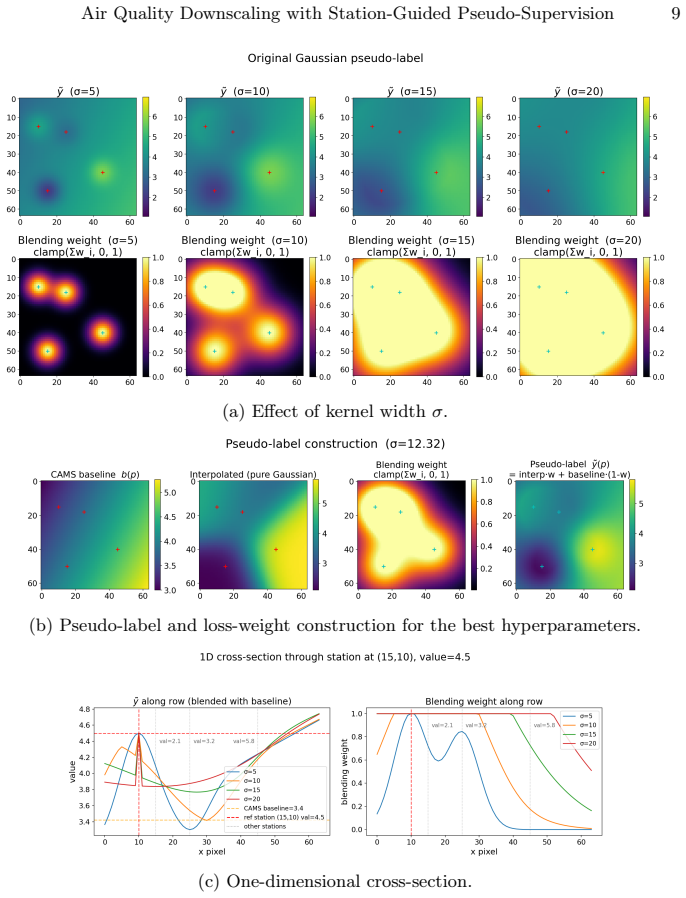
The STARQ framework consists of three components: (1) a SegFormer-based four-stage hierarchical transformer encoder that processes multi-channel geospatial raster inputs, producing multi-scale features that are fused and upsampled to 1 km resolution; (2) Gaussian-kernel pseudo-label propagation (Eqs. 1-4), where each station's influence decays isotropically with a fixed standard deviation (σ=12.32 pixels), and a cumulative confidence map blends station-interpolated values with the CAMS baseline depending on local station density; and (3) a dual training objective (Eq. 8) combining direct station-level MSE loss with dense pseudo-label MSE loss over non-station pixels, weighted by λ_s=0.173, λ
Load-bearing premise
The pseudo-labels that supervise the network on non-station pixels are constructed by spreading station measurements with a fixed isotropic Gaussian kernel (σ=12.32 pixels) and blending with the CAMS baseline where stations are sparse. If real PM2.5 spatial structure is anisotropic (driven by wind transport, topographic channeling, or sharp urban-rural gradients), these pseudo-labels will be systematically wrong and the model will learn to reproduce those errors.
What would settle it
If the Gaussian-blended pseudo-labels are essential, then training with only station-level loss (no pseudo-label loss) should substantially degrade performance. If the pseudo-labels are not essential, the transformer may achieve similar results using only station-level supervision plus the auxiliary geospatial inputs, which would undermine the central methodological contribution.
If this is right
- If the Gaussian-kernel propagation approach generalizes, it could be applied to other environmental downscaling problems where sparse point observations must supervise dense spatial predictions, such as soil moisture, ozone, or temperature fields.
- The time-agnostic design means operational air-quality systems could produce 1 km PM2.5 maps at arbitrary timestamps without maintaining temporal model state, potentially simplifying deployment in real-time public health alerting systems.
- The finding that CAMS PM2.5 and built-up surface features dominate channel importance suggests that urban morphology is a primary driver of fine-scale PM2.5 variability, and future downscaling efforts may benefit from prioritizing high-resolution urban form data over additional meteorological inputs.
- The consistent improvements across land-use categories, including the large gain in water-covered regions, indicate that explicit spatial context modeling captures pollutant-land-surface interactions that point-wise regression methods miss.
Where Pith is reading between the lines
- The fixed isotropic Gaussian kernel (σ=12.32 pixels) cannot represent anisotropic pollutant transport along wind corridors or topographic channeling, yet the model still improves substantially — this suggests the transformer learns to override pseudo-label errors using side information, raising the question of whether the pseudo-labels are load-bearing or whether the network could be trained with
- If the pseudo-label mechanism is the key contribution, then regions with very sparse station coverage (rural, remote) would have pseudo-labels dominated by the CAMS baseline, meaning the model's corrections in those regions are essentially learning to reproduce CAMS — the R² gains may be concentrated in station-dense urban areas, which would limit the practical value for exposure assessment in und
- The spatiotemporal split evaluates on unseen stations but within the same geographic domain; the approach may not transfer to regions with fundamentally different station networks or pollution regimes, since the network may be learning region-specific station-CAMS bias patterns rather than generalizable spatial relationships.
Editorial analysis
A structured set of objections, weighed in public.
Referee Report
Summary. This paper presents STARQ, a SegFormer-based framework for downscaling CAMS PM2.5 forecasts from 0.4° to 0.01° (~1 km) over Europe. The method introduces a Gaussian-kernel pseudo-label propagation scheme that blends station-interpolated values with the CAMS baseline to provide dense supervision from sparse OpenAQ station observations. The model is trained from scratch on eight heterogeneous geospatial and atmospheric input channels, without temporal sequence modeling. Evaluation is conducted under a spatiotemporal split (unseen timestamps and unseen stations), and STARQ is compared against the CAMS baseline and S-MESH*, an XGBoost-based downscaling method. The authors report improvements in MAE, RMSE, and R² across multiple land-use categories, and provide channel-importance analyses and qualitative visualizations.
Significance. The paper addresses a practically important problem: producing high-resolution, bias-corrected PM2.5 fields at continental scale from coarse operational forecasts and sparse ground observations. The time-agnostic formulation is a reasonable design choice that allows single-timestamp inference. The spatiotemporal evaluation protocol (holding out both stations and timestamps) is rigorous and appropriate for assessing generalization. The channel-importance analysis using three complementary methods (ablation, gradient sensitivity, permutation) is a strength. The continental-scale scope and the 40× downscaling factor are notable. However, the significance of the results is tempered by the modest absolute R² (0.242) and by a missing baseline that would isolate the neural network's contribution from the Gaussian interpolation it is trained to reproduce.
major comments (3)
- §4.2, Eqs. (4) and (7); §5, Table 2: The paper does not report the pseudo-label field y_pseudo(p) itself as a baseline at held-out test stations. Since the model is trained with λ_p=0.970 dominating λ_s=0.173, the network's behavior at non-station pixels is strongly shaped by the Gaussian interpolation blended with CAMS. If the pseudo-label field constructed from training stations alone already achieves MAE/R² comparable to STARQ's reported numbers at test station locations, the neural network's learned contribution would be marginal. This baseline is essential to distinguish STARQ's learned spatial structure from the interpolation it is trained to reproduce. The authors should compute y_pseudo at held-out test station locations (using only training stations for the Gaussian interpolation) and report its MAE/R² alongside Table 2.
- §5, Table 2: No ablation isolating the contribution of the pseudo-label propagation scheme itself is reported. For instance, training the same SegFormer architecture with only L_station (λ_p=0) would show whether the pseudo-label supervision is load-bearing for the reported improvements, or whether the network learns the mapping from side information to station-level PM2.5 independently. Without this, the central methodological contribution is not properly assessed.
- §4.2, Eq. (3): The cumulative station-confidence map W(p) = max(0, min(1, Σ w_i(p))) is a sum of unnormalized Gaussian weights. For a pixel near multiple stations, this sum can exceed 1 and is clamped, but for a pixel near a single station at moderate distance, W(p) can be very small, causing the pseudo-label to default to the CAMS baseline b(p). The sensitivity of downstream results to this confidence mapping is not discussed. The authors should either justify this specific functional form or report sensitivity to alternative normalizations (e.g., W(p) = max_i w_i(p) or a softmax-based weighting).
minor comments (7)
- §5.1: The model is trained with RMSE loss (Eq. 7 uses squared error) but the best checkpoint is selected by lowest validation MAE. This mismatch should be noted and justified.
- Table 3: The 'No Data/Unknown' category has N=1,105 and very high MAE (15.222 for STARQ). This small, anomalous category may distort aggregate metrics. Consider reporting overall metrics with and without this category.
- §5.3, Fig. 7: MODIS AOD and GHSL population show slightly negative importance in ablation/permutation. The paper briefly attributes this to noise or redundancy, but given that AOD is a commonly used predictor in PM2.5 downscaling literature, a more thorough discussion would strengthen the analysis.
- §3: The Italian dataset used for hyperparameter tuning is described as covering 2018, 2020, and 2023, but the temporal extent of the full European dataset is not specified. This should be stated.
- Fig. 6: The two time-series case studies are on validation stations, not test stations. If available, showing test-station time series would be more convincing of generalization.
- §4.2, Eq. (1): The Gaussian kernel uses σ=12.32 pixels (tuned on the Italian dataset). It would help to state the physical distance this corresponds to (approximately 12.32 km at 0.01° resolution) for interpretability.
- The paper mentions 'S-MESH*' as their implementation of S-MESH [49], but details of this implementation (feature set, hyperparameters, training data) are not provided in the main text. A brief description or reference to supplementary material would aid reproducibility.
Simulated Author's Rebuttal
We thank the referee for a careful and constructive review. The referee correctly identifies that the pseudo-label baseline and the pseudo-label ablation are critical missing experiments, and we agree these must be added. We also provide a substantive response on the confidence-map design question.
read point-by-point responses
-
Referee: Comment 1 (§4.2, Eqs. (4) and (7); §5, Table 2): Report y_pseudo at held-out test stations as a baseline, using only training stations for the Gaussian interpolation, to distinguish STARQ's learned contribution from the interpolation it is trained to reproduce.
Authors: The referee is correct that this baseline is essential and currently missing from the manuscript. We will compute y_pseudo at held-out test station locations—constructing the Gaussian interpolation using only training stations—and report its MAE/R² alongside Table 2 in the revised manuscript. We expect this baseline to underperform STARQ for the following reason: the pseudo-label field is a blend of station interpolation and the CAMS prior, so at test station locations (which are unseen during training), the pseudo-label defaults to the CAMS baseline wherever training-station support is weak. Since test stations are held out, the Gaussian interpolation cannot directly leverage their observations. STARQ, by contrast, learns spatial relationships from side information (land use, elevation, population, wind, etc.) that generalize to unseen station locations. The network's contribution is precisely to predict PM2.5 at locations where station support is absent, using learned environmental correlations rather than direct interpolation. Nevertheless, we agree this must be demonstrated empirically rather than argued a priori. revision: yes
-
Referee: Comment 2 (§5, Table 2): Report an ablation isolating the pseudo-label propagation scheme (e.g., training with only L_station, λ_p=0) to assess whether pseudo-label supervision is load-bearing for the reported improvements.
Authors: We agree this ablation is necessary to properly assess the central methodological contribution. We will train the same SegFormer architecture with only L_station (λ_p=0) and report the resulting metrics alongside Table 2. We note that training with only station-level supervision on sparse point observations is a fundamentally ill-posed dense prediction problem: the network receives gradient signal at only a handful of pixel locations per patch, with no supervision elsewhere. This makes optimization unstable and prone to trivial solutions (e.g., reproducing the CAMS prior everywhere except at station pixels). The pseudo-label propagation scheme was designed precisely to address this sparsity by providing dense supervision. However, the referee is right that this design rationale must be validated experimentally, and we will include the ablation in the revision. revision: yes
-
Referee: Comment 3 (§4.2, Eq. (3): Sensitivity of results to the confidence map W(p) = max(0, min(1, Σ w_i(p))), including comparison to alternatives such as max_i w_i(p) or softmax-based weighting.
Authors: We appreciate this observation. The referee correctly notes that the cumulative sum formulation causes W(p) to saturate (clamp to 1) near station clusters while remaining small near isolated stations, causing the pseudo-label to default to CAMS in the latter case. This is actually a deliberate design property: in regions with dense station coverage, we trust the interpolation; in regions with sparse coverage, we fall back to the CAMS prior, which is physically informed. An alternative like W(p) = max_i w_i(p) would treat single-station and multi-station support identically, discarding the signal that a pixel is corroborated by multiple stations. That said, we acknowledge that this design choice was not justified in the manuscript, nor was its sensitivity to alternatives assessed. We will (a) add a paragraph in §4.2 explaining the rationale for the cumulative-sum formulation, and (b) run a sensitivity experiment comparing against W(p) = max_i w_i(p) on the Italian validation dataset, reporting the results in the revised manuscript. If the alternative formulation yields comparable or better performance, we will report this transparently. revision: partial
Circularity Check
No significant circularity: the pseudo-label construction is a training-time interpolation scheme, not a fitted parameter renamed as prediction; the model is evaluated against held-out ground truth it never saw.
specific steps
-
self definitional
[Eq. 4 (Section 4.2) and Eq. 7]
"ypseudo(p) = W(p)˜y(p) + (1−W(p))b(p). (4) ... Lpseudo = 1/|Ω∖S| Σ_{p∈Ω∖S} (ŷ(p) − ypseudo(p))² (7)"
The pseudo-label y_pseudo (Eq. 4) blends Gaussian-interpolated station values ỹ(p) with the CAMS baseline b(p), and L_pseudo (Eq. 7) trains the model to reproduce y_pseudo at non-station pixels. Since b(p) = CAMS is also a model input, in station-sparse regions where W(p)→0 the supervision target approaches b(p), meaning the model is trained to reproduce its own input. This is a mild structural circularity: the model is partly supervised by its own input in sparse regions. However, this is not a fatal circularity because (1) at and near stations W(p)→1 and the target is station-interpolated values, not CAMS; (2) the model also receives L_station on held-out training stations; (3) evaluation is on spatiotemporally held-out test stations where the model must generalize beyond both the pseudo
-
fitted input called prediction
[Section 5.1, hyperparameter σ=12.32 pixels; Table 2 evaluation]
"The best configuration, subsequently used also on the full European dataset, consisted of ... a Gaussian standard deviation of σ= 12.32 pixels, as well as station- and pseudo-label-supervision weights of λs = 0.173 and λp = 0.970"
σ was tuned on the Italian dataset to minimize validation MAE, then applied to the European dataset. The pseudo-label field constructed with this σ is the dominant training target (λ_p=0.970 ≫ λ_s=0.173). The paper does not report the pseudo-label field itself as a baseline at held-out test stations, so one cannot fully separate how much of STARQ's test performance comes from the network learning genuine spatial structure versus reproducing the Gaussian interpolation that was tuned to minimize station-level error. This is a methodological gap rather than a strict circularity: the model is not evaluated on the same data used to fit σ, and the test stations are genuinely held out. The concern is about attribution of improvement, not about the result being forced by construction.
full rationale
The paper's central claim — that STARQ outperforms CAMS and S-MESH* on held-out test stations — is not circularly forced. The evaluation uses a strict spatiotemporal split (unseen timestamps and unseen stations), and the model is compared against ground truth it never observed during training. The two circularity-adjacent issues are: (1) the pseudo-label target (Eq. 4) blends station interpolation with the CAMS baseline, which is also a model input, creating a mild self-referential loop in station-sparse regions; and (2) the Gaussian kernel width σ was tuned on a separate Italian dataset and the pseudo-label field itself is not reported as a baseline, making it difficult to fully attribute STARQ's gains to the network versus the interpolation prior. Neither issue reduces the claimed test-set results to the inputs by construction. The model could still fail to generalize — the improvement is not guaranteed by the setup. Score 2 reflects these minor structural concerns without rising to the level where predictions are forced by definition or fit.
Axiom & Free-Parameter Ledger
free parameters (11)
- σ (Gaussian kernel width) =
12.32 pixels
- λ_s (station loss weight) =
0.173
- λ_p (pseudo-label loss weight) =
0.970
- learning rate =
1.31e-5
- weight decay =
1.95e-5
- background sampling ratio =
0.176
- SegFormer hidden dimensions =
[256, 512, 1280, 2048]
- SegFormer transformer depths =
[3, 8, 27, 3]
- bucket size K =
4
- patch size =
64×64
- fading width F =
O/2
axioms (5)
- domain assumption Gaussian kernel interpolation adequately represents the spatial structure of PM2.5 between monitoring stations
- domain assumption CAMS forecasts provide a physically consistent spatial prior that is locally biased but structurally informative
- domain assumption OpenAQ station measurements are accurate ground truth for PM2.5
- domain assumption SegFormer architecture is suitable for multi-channel geospatial raster regression
- domain assumption Hyperparameters tuned on the Italian dataset transfer to the full European domain
read the original abstract
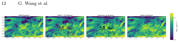
Super-resolving coarse atmospheric fields to local PM$_{2.5}$ variations is uniquely challenged by a mismatch in spatial support: while pixels represent regional averages, ground-truth observations are discrete, unaligned samples of a continuous spatial signal. To bridge this gap, we present a station-guided framework for high-resolution PM$_{2.5}$ downscaling over Europe. Taking coarse CAMS atmospheric composition fields alongside heterogeneous side information (i.e., human activity, land cover, elevation, satellite aerosol observations, and wind fields) our framework jointly super-resolves ($\times 40$, $\approx$ 1 km) and bias-corrects CAMS rasters, without relying on temporal sequence modelling. To address the challenge of densely supervising our multi-scale transformer network with sparse in-situ data, we introduce a time-agnostic propagation strategy that utilises spatial Gaussian blending of interpolated OpenAQ observations. Extensive qualitative and station-level evaluations across Europe demonstrate that our model recovers fine-grained spatial structures and effectively mitigates localised CAMS biases.
Figures




Reference graph
Works this paper leans on
-
[1]
OpenAQ : Retrieved from https://api.openaq.org .https://api.openaq.org (2023)
work page 2023
-
[2]
Ashiotis, G., Tsigkanos, E., Christoudias, T., Nicolaou, M.A.: Ai for air qual- ity: Leveraging data fusion for deep downscaling of atmospheric pollutants. In: MACLEAN@ PKDD/ECML (2022)
work page 2022
-
[3]
Geoscientific Model Development13(4), 2109–2124 (2020)
Baño-Medina, J., Manzanas, R., Gutiérrez, J.M.: Configuration and intercompari- son of deep learning neural models for statistical downscaling. Geoscientific Model Development13(4), 2109–2124 (2020)
work page 2020
-
[4]
Nature619(7970), 533–538 (2023)
Bi, K., Xie, L., Zhang, H., Chen, X., Gu, X., Tian, Q.: Accurate medium-range global weather forecasting with 3d neural networks. Nature619(7970), 533–538 (2023)
work page 2023
- [5]
-
[6]
Communications Earth & Environment6(1), 518 (2025)
Chen, K., Han, T., Ling, F., Gong, J., Bai, L., Wang, X., Luo, J.J., Fei, B., Zhang, W., Chen, X., et al.: The operational medium-range deterministic weather fore- casting can be extended beyond a 10-day lead time. Communications Earth & Environment6(1), 518 (2025)
work page 2025
-
[7]
npj climate and atmospheric science6(1), 190 (2023)
Chen, L., Zhong, X., Zhang, F., Cheng, Y., Xu, Y., Qi, Y., Li, H.: Fuxi: a cascade machine learning forecasting system for 15-day global weather forecast. npj climate and atmospheric science6(1), 190 (2023)
work page 2023
-
[8]
Chen, T., Guestrin, C.: Xgboost: A scalable tree boosting system. In: Proceedings of the 22nd acm sigkdd international conference on knowledge discovery and data mining. pp. 785–794 (2016)
work page 2016
-
[9]
Copernicus Atmosphere Monitoring Service (CAMS): Cams european air quality reanalyses. Copernicus Atmosphere Monitoring Service (CAMS) Atmosphere Data Store (2021).https://doi.org/10.24381/7cc0465a,https://ads.atmosphere. copernicus.eu/cdsapp#!/dataset/cams-europe-air-quality-reanalyses, ac- cessed on 25-Oct-2025
-
[10]
Copernicus Atmosphere Monitoring Service (CAMS): Cams global atmospheric composition forecasts. Copernicus Atmosphere Monitoring Service (CAMS) Atmo- sphere Data Store (2021).https://doi.org/10.24381/04a0b097,https://ads. atmosphere . copernicus . eu / cdsapp # ! / dataset / cams - global - atmospheric - composition-forecasts, accessed on 25-Oct-2025
-
[11]
Copernicus Atmosphere Monitoring Service (CAMS): Cams assessment report on european air quality in 2024.https://atmosphere.copernicus.eu/node/1330 (2025), doi:10.24380/pdtn-dc12
-
[12]
Copernicus Land Monitoring Service: Corine land cover 2018 (raster 100 m), eu- rope, 6-yearly – version 2020_20u1, may 2020 (2020).https://doi.org/10.2909/ 960998c1- 1870- 4e82- 8051- 6485205ebbac,https://land.copernicus.eu/en/ products/corine-land-cover/clc2018, european Union’s Copernicus Land Mon- itoring Service information. Accessed on 01.11.2025
work page 2018
-
[13]
Ocean engineering26(3), 191–203 (1998)
Deo, M., Naidu, C.S.: Real time wave forecasting using neural networks. Ocean engineering26(3), 191–203 (1998)
work page 1998
-
[14]
Eskes, H., Tsikerdekis, A., Ades, M., Alexe, M., Benedictow, A.C., Bennouna, Y., Blake, L., Bouarar, I., Chabrillat, S., Engelen, R., et al.: Evaluation of the coper- nicus atmosphere monitoring service cy48r1 upgrade of june 2023. Atmospheric Chemistry and Physics24(16), 9475–9514 (2024) Air Quality Downscaling with Station-Guided Pseudo-Supervision 17
work page 2023
-
[15]
Geoscientific Model Development15(17), 6677–6694 (2022)
Geiss, A., Silva, S.J., Hardin, J.C.: Downscaling atmospheric chemistry simulations with physically consistent deep learning. Geoscientific Model Development15(17), 6677–6694 (2022)
work page 2022
-
[16]
GISCO, E.: European digital elevation model (eu-dem), version 1.1. Dataset down- loaded from Eurostat GISCO website (2016),https://ec.europa.eu/eurostat/ web/gisco/geodata/digital-elevation-model/eu-dem, accessed 2025-11-02
work page 2016
-
[17]
American Heart Journal Plus: Cardiology Research and Practice25, 100231 (2023)
Goldsborough III, E., Gopal, M., McEvoy, J.W., Blumenthal, R.S., Jacobsen, A.P.: Pollution and cardiovascular health: a contemporary review of morbidity and im- plications for planetary health. American Heart Journal Plus: Cardiology Research and Practice25, 100231 (2023)
work page 2023
-
[18]
5 and pm10 hourly concentrations in a euro- pean air quality hotspot
Gualtieri, G., Brilli, L., Carotenuto, F., Cavaliere, A., Gioli, B., Giordano, T., Putzolu, S., Vagnoli, C., Zaldei, A.: Assessing capability of copernicus atmosphere monitoring service to forecast pm2. 5 and pm10 hourly concentrations in a euro- pean air quality hotspot. Atmospheric Pollution Research p. 102567 (2025)
work page 2025
-
[19]
Guion, A., Gressent, A., Descombes, G., Janati, Y., Real, E., Ung, A., Meleux, F., Schucht, S., Colette, A.: High-resolution mapping of air quality across europe: an ensemble machine and deep learning framework integrating multi-scale spatial predictors (chromap v1. 0). EGUsphere2026, 1–35 (2026)
work page 2026
-
[20]
FengWu-GHR: Learning the Kilometer-scale Medium-range Global Weather Forecasting
Han,T.,Guo,S.,Ling,F.,Chen,K.,Gong,J.,Luo,J.,Gu,J.,Dai,K.,Ouyang,W., Bai, L.: Fengwu-ghr: Learning the kilometer-scale medium-range global weather forecasting. arXiv preprint arXiv:2402.00059 (2024)
work page internal anchor Pith review Pith/arXiv arXiv 2024
-
[21]
Geophysical Research Letters50(24), e2023GL104928 (2023)
Han, W., He, T.L., Jiang, Z., Zhu, R., Jones, D., Miyazaki, K., Shen, Y.: The capability of deep learning model to predict ozone across continents in china, the united states and europe. Geophysical Research Letters50(24), e2023GL104928 (2023)
work page 2023
-
[22]
Hersbach, H., Bell, B., Berrisford, P., Biavati, G., Horanyi, A., Munoz Sabater, J., Nicolas, J., Peubey, C., Radu, R., Rozum, I., Schepers, D., Simmons, A., Soci, C., Dee, D., Thepaut, J.N.: Era5 hourly data on single levels from 1940 to present (2023).https://doi.org/10.24381/cds.adbb2d47,https://doi.org/10.24381/ cds.adbb2d47, generated using or contai...
-
[23]
5 forecasting: Mk hossen et al
Hossen, M.K., Peng, Y.T., Shao, A., Chen, M.C.: An ode based neural network approach for pm2. 5 forecasting: Mk hossen et al. Scientific Reports15(1), 24830 (2025)
work page 2025
-
[24]
Hsieh, W.W., Tang, B.: Applying neural network models to prediction and data analysisinmeteorologyandoceanography.BulletinoftheAmericanMeteorological Society79(9), 1855–1870 (1998)
work page 1998
-
[25]
Atmospheric Chemistry and Physics19, 3515–3556 (2019).https://doi.org/10
Inness, A., Ades, M., Agustí-Panareda, A., Barré, J., Benedictow, A., Blech- schmidt, A.M., Dominguez, J.J., Engelen, R., Eskes, H., Flemming, J., Huijnen, V., Jones, L., Kipling, Z., Massart, S., Parrington, M., Peuch, V.H., Razinger, M., Remy, S., Schulz, M., Suttie, M.: The cams reanalysis of atmospheric composition. Atmospheric Chemistry and Physics19...
-
[26]
Environmental Moni- toring and Assessment65(1), 277–286 (2000)
Kolehmainen, M., Martikainen, H., Hiltunen, T., Ruuskanen, J.: Forecasting air quality parameters using hybrid neural network modelling. Environmental Moni- toring and Assessment65(1), 277–286 (2000)
work page 2000
-
[27]
5 forecast model combining convlstm and dnn in seoul
Koo, J.S., Wang, K.H., Yun, H.Y., Kwon, H.Y., Koo, Y.S.: Development of pm2. 5 forecast model combining convlstm and dnn in seoul. Atmosphere15(11), 1276 (2024) 18 G. Wang et al
work page 2024
-
[28]
Monthly weather review126(2), 470–482 (1998)
Kuligowski, R.J., Barros, A.P.: Experiments in short-term precipitation forecasting using artificial neural networks. Monthly weather review126(2), 470–482 (1998)
work page 1998
-
[29]
Science382(6677), 1416–1421 (2023)
Lam, R., Sanchez-Gonzalez, A., Willson, M., Wirnsberger, P., Fortunato, M., Alet, F., Ravuri, S., Ewalds, T., Eaton-Rosen, Z., Hu, W., et al.: Learning skillful medium-range global weather forecasting. Science382(6677), 1416–1421 (2023)
work page 2023
-
[30]
Scientific Reports15(1), 38616 (2025)
Lee, Y., Park, J., Kim, J., Woo, J.H., Lee, J.H.: Conditional unet emulation of cmaq simulations for fine particulate matter concentration prediction. Scientific Reports15(1), 38616 (2025)
work page 2025
-
[31]
Journal of Applied Meteorology and Climatology57(10), 2267– 2283 (2018)
Liu, D., Grimmond, C., Tan, J., Ao, X., Peng, J., Cui, L., Ma, B., Hu, Y., Du, M.: A new model to downscale urban and rural surface and air temperatures evaluated in shanghai, china. Journal of Applied Meteorology and Climatology57(10), 2267– 2283 (2018)
work page 2018
-
[32]
Lv, B., Hu, Y., Chang, H.H., Russell, A.G., Cai, J., Xu, B., Bai, Y.: Daily es- timation of ground-level pm2. 5 concentrations at 4 km resolution over beijing- tianjin-hebei by fusing modis aod and ground observations. Science of the Total Environment580, 235–244 (2017)
work page 2017
-
[33]
Lyapustin, A., Wang, Y.: Modis/terra+aqua land aerosol optical depth daily l2g global 1km sin grid v061 (2022).https://doi.org/10.5067/MODIS/MCD19A2.061, https://doi.org/10.5067/MODIS/MCD19A2.061
-
[34]
Journal of Applied Meteorology and Climatology 35(5), 617–626 (1996)
Marzban, C., Stumpf, G.J.: A neural network for tornado prediction based on doppler radar-derived attributes. Journal of Applied Meteorology and Climatology 35(5), 617–626 (1996)
work page 1996
-
[35]
Weather and Forecasting7(3), 525–534 (1992)
McCann, D.W.: A neural network short-term forecast of significant thunderstorms. Weather and Forecasting7(3), 525–534 (1992)
work page 1992
-
[36]
International Journal of Geographical Information System 4(3), 313–332 (1990)
Oliver, M.A., Webster, R.: Kriging: a method of interpolation for geographical information systems. International Journal of Geographical Information System 4(3), 313–332 (1990)
work page 1990
-
[37]
OpenAI, R.: Gpt-4 technical report. arxiv 2303.08774. View in Article2(5), 1 (2023)
work page internal anchor Pith review Pith/arXiv arXiv 2023
-
[38]
5 and PM10), ozone, nitrogen dioxide, sulfur dioxide and carbon monoxide
Organization, W.H., et al.: WHO global air quality guidelines: particulate matter (PM2. 5 and PM10), ozone, nitrogen dioxide, sulfur dioxide and carbon monoxide. World Health Organization (2021)
work page 2021
-
[39]
europa.eu/89h/9f06f36f-4b11-47ec-abb0-4f8b7b1d72ea
Pesaresi, M., Politis, P.: Ghs-built-s r2023a - ghs built-up surface grid, derived from sentinel2 composite and landsat, multitemporal (1975–2030) (2023).https: //doi.org/10.2905/9F06F36F- 4B11- 47EC- ABB0- 4F8B7B1D72EA,http://data. europa.eu/89h/9f06f36f-4b11-47ec-abb0-4f8b7b1d72ea
-
[40]
Pesaresi, M., Politis, P.: Ghs-built-v r2023a - ghs built-up volume grids de- rived from joint assessment of sentinel2, landsat, and global dem data, mul- titemporal (1975–2030) (2023).https : / / doi . org / 10 . 2905 / AB2F107A - 03CD - 47A3-85E5-139D8EC63283,http://data.europa.eu/89h/ab2f107a-03cd-47a3- 85e5 - 139d8ec63283, pID: http://data.europa.eu/8...
work page 1975
-
[41]
5 prediction using imputed maiac aod with un- certainty quantification
Pu, Q., Yoo, E.H.: Ground pm2. 5 prediction using imputed maiac aod with un- certainty quantification. Environmental Pollution274, 116574 (2021)
work page 2021
-
[42]
npj Climate and Atmospheric Science6(1), 71 (2023)
Qiu, Y., Feng, J., Zhang, Z., Zhao, X., Li, Z., Ma, Z., Liu, R., Zhu, J.: Regional aerosol forecasts based on deep learning and numerical weather prediction. npj Climate and Atmospheric Science6(1), 71 (2023)
work page 2023
-
[43]
Rautela, K.S., Goyal, M.K., Nagpure, A.S.: Unequal spatio-temporal distribution of population-weighted pollution extremes through deep learning. npj Climate and Atmospheric Science8(1), 340 (2025) Air Quality Downscaling with Station-Guided Pseudo-Supervision 19
work page 2025
-
[44]
In: International Conference on Medical image computing and computer-assisted intervention
Ronneberger, O., Fischer, P., Brox, T.: U-net: Convolutional networks for biomedi- cal image segmentation. In: International Conference on Medical image computing and computer-assisted intervention. pp. 234–241. Springer (2015)
work page 2015
-
[45]
nature323(6088), 533–536 (1986)
Rumelhart, D.E., Hinton, G.E., Williams, R.J.: Learning representations by back- propagating errors. nature323(6088), 533–536 (1986)
work page 1986
-
[46]
Schiavina, M., Freire, S., Carioli, A., MacManus, K.: Ghs-pop r2023a - ghs population grid multitemporal (1975–2030) (2023).https : / / doi . org / 10 . 2905 / 2FF68A52 - 5B5B - 4A22 - 8F40 - C41DA8332CFE,http : / / data . europa . eu / 89h / 2ff68a52 - 5b5b - 4a22 - 8f40 - c41da8332cfe, pID: http://data.europa.eu/89h/2ff68a52-5b5b-4a22-8f40-c41da8332cfe
work page 1975
-
[47]
Shen, H., Tao, S., Chen, Y., Ciais, P., Güneralp, B., Ru, M., Zhong, Q., Yun, X., Zhu, X., Huang, T., et al.: Urbanization-induced population migration has reduced ambient pm2. 5 concentrations in china. Science Advances3(7), e1700300 (2017)
work page 2017
-
[48]
Scientific reports4(1), 6561 (2014)
Shen, H., Tao, S., Liu, J., Huang, Y., Chen, H., Li, W., Zhang, Y., Chen, Y., Su, S., Lin, N., et al.: Global lung cancer risk from pah exposure highly depends on emission sources and individual susceptibility. Scientific reports4(1), 6561 (2014)
work page 2014
-
[49]
5 estimation over europe by ml- based downscaling of the cams regional forecast
Shetty, S., Hamer, P.D., Stebel, K., Kylling, A., Hassani, A., Berntsen, T.K., Schneider, P.: Daily high-resolution surface pm2. 5 estimation over europe by ml- based downscaling of the cams regional forecast. Environmental Research264, 120363 (2025)
work page 2025
-
[50]
Science advances7(3), eabd6696 (2021)
Shi, Z., Song, C., Liu, B., Lu, G., Xu, J., Van Vu, T., Elliott, R.J., Li, W., Bloss, W.J., Harrison, R.M.: Abrupt but smaller than expected changes in surface air quality attributable to covid-19 lockdowns. Science advances7(3), eabd6696 (2021)
work page 2021
-
[51]
Atmospheric Environment32(24), 4195–4206 (1998)
Sørensen, J.H.: Sensitivity of the derma long-range gaussian dispersion model to meteorological input and diffusion parameters. Atmospheric Environment32(24), 4195–4206 (1998)
work page 1998
-
[52]
Applied Geography19(2), 123–136 (1999)
Spellman, G.: An application of artificial neural networks to the prediction of surface ozone concentrations in the united kingdom. Applied Geography19(2), 123–136 (1999)
work page 1999
-
[53]
Climate Dynamics13(2), 135–147 (1997)
Tangang, F., Hsieh, W., Tang, B.: Forecasting the equatorial pacific sea surface temperatures by neural network models. Climate Dynamics13(2), 135–147 (1997)
work page 1997
-
[54]
5 by hybrid graph deep neural network with aggregated neighborhood spatiotemporal information
Teng, M., Li, S., Xing, J., Fan, C., Yang, J., Wang, S., Song, G., Ding, Y., Dong, J., Wang, S.: 72-hour real-time forecasting of ambient pm2. 5 by hybrid graph deep neural network with aggregated neighborhood spatiotemporal information. Environment International176, 107971 (2023)
work page 2023
-
[55]
Atmospheric Chemistry and Physics12(12), 5447–5481 (2012)
Tørseth, K., Aas, W., Breivik, K., Fjæraa, A.M., Fiebig, M., Hjellbrekke, A.G., Lund Myhre, C., Solberg, S., Yttri, K.E.: Introduction to the european monitoring and evaluation programme (emep) and observed atmospheric composition change during 1972–2009. Atmospheric Chemistry and Physics12(12), 5447–5481 (2012)
work page 1972
-
[56]
5 predictions from cams air quality models to urban monitoring sites in budapest
Varga-Balogh, A., Leelőssy, Á., Lagzi, I., Mészáros, R.: Time-dependent downscal- ing of pm2. 5 predictions from cams air quality models to urban monitoring sites in budapest. Atmosphere11(6), 669 (2020)
work page 2020
-
[57]
Advances in neural information pro- cessing systems30(2017)
Vaswani,A.,Shazeer,N.,Parmar,N.,Uszkoreit,J.,Jones,L.,Gomez,A.N.,Kaiser, Ł., Polosukhin, I.: Attention is all you need. Advances in neural information pro- cessing systems30(2017)
work page 2017
-
[58]
Water Resources Research57(4), e2020WR029308 (2021)
Wang, F., Tian, D., Lowe, L., Kalin, L., Lehrter, J.: Deep learning for daily precipitation and temperature downscaling. Water Resources Research57(4), e2020WR029308 (2021)
work page 2021
-
[59]
PNAS nexus 4(6), pgaf198 (2025) 20 G
Wang, Y., Fernández-Godino, M.G., Gunawardena, N., Lucas, D.D., Yue, X.: Spa- tiotemporal predictions of toxic urban plumes using deep learning. PNAS nexus 4(6), pgaf198 (2025) 20 G. Wang et al
work page 2025
-
[60]
Fine-grained prediction of reading comprehension from eye movements,
Wolf, T., Debut, L., Sanh, V., Chaumond, J., Delangue, C., Moi, A., Cistac, P., Rault, T., Louf, R., Funtowicz, M., Davison, J., Shleifer, S., von Platen, P., Ma, C., Jernite, Y., Plu, J., Xu, C., Le Scao, T., Gugger, S., Drame, M., Lhoest, Q., Rush, A.: Transformers: State-of-the-art natural language processing. In: Liu, Q., Schlangen, D. (eds.) Proceedi...
-
[61]
Xiao, Y., Wang, Y., Yuan, Q., He, J., Zhang, L.: Generating a long-term (2003-
work page 2003
-
[62]
5 dataset via spatiotemporal downscaling of cams with deep learning (deepcams)
hourly 0.25°global pm2. 5 dataset via spatiotemporal downscaling of cams with deep learning (deepcams). Science of The Total Environment848, 157747 (2022)
work page 2022
-
[63]
Advances in neural information processing systems34, 12077–12090 (2021)
Xie, E., Wang, W., Yu, Z., Anandkumar, A., Alvarez, J.M., Luo, P.: Segformer: Simple and efficient design for semantic segmentation with transformers. Advances in neural information processing systems34, 12077–12090 (2021)
work page 2021
-
[64]
Xue, T., Zheng, Y., Tong, D., Zheng, B., Li, X., Zhu, T., Zhang, Q.: Spatiotemporal continuous estimates of pm2. 5 concentrations in china, 2000–2016: A machine learning method with inputs from satellites, chemical transport model, and ground observations. Environment international123, 345–357 (2019)
work page 2000
-
[65]
Yang, Q., Yuan, Q., Li, T., Yue, L.: Mapping pm2. 5 concentration at high res- olution using a cascade random forest based downscaling model: Evaluation and application. Journal of Cleaner Production277, 123887 (2020) Air Quality Downscaling with Station-Guided Pseudo-Supervision 21 Supplementary Material A Additional Data Processing Details A.1 Side Info...
work page 2020
discussion (0)
Sign in with ORCID, Apple, or X to comment. Anyone can read and Pith papers without signing in.