REVIEW 2 major objections 5 minor 66 references
Krylov complexity is the leading derivative of a Loschmidt amplitude under an angular Hamiltonian deformation, and is upper-bounded by the volume of the resulting two-dimensional quantum geometry.
Reviewed by Pith at T0; open to challenge. T0 means a machine referee read the full paper against a public rubric. the ladder, T0–T4 →
T0 review · grok-4.5
2026-07-14 08:16 UTC pith:HFREJQEM
load-bearing objection Clean algebraic rewrite of Krylov complexity as a Loschmidt derivative plus a volume bound; soft spots are the non-rigorous approximate inequalities, not the core claims. the 2 major comments →
Krylov Complexity from Loschmidt Amplitude
The pith
A machine-rendered reading of the paper's core claim, the machinery that carries it, and where it could break.
Core claim
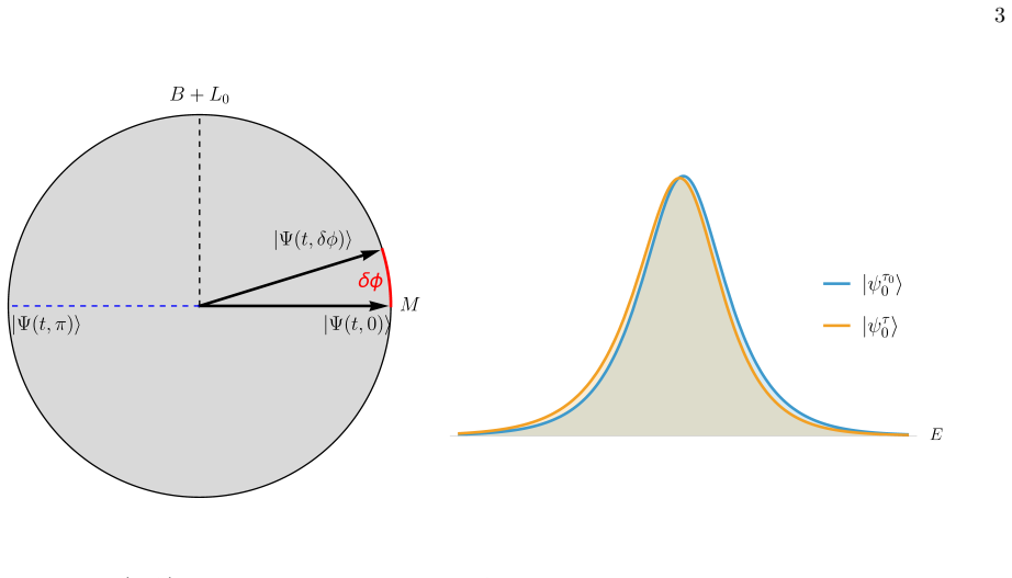
Krylov complexity equals the leading φ-derivative of the Loschmidt amplitude G(t,φ)=⟨0|e^{iMt}e^{-iM(φ)t}|0⟩, where M(φ) is the Hamiltonian rotated by the Krylov number operator; the same complexity is always upper-bounded by the volume of the two-dimensional (t,φ) geometry induced by the Fubini-Study metric.
What carries the argument
The φ-rotated Hamiltonian M(φ)=M cos φ + B sin φ + L_0(1-cos φ), together with the associated spectral Poisson kernel K(E1,E2,φ) that propagates the Krylov number operator in the energy basis; its φ-derivatives generate every moment of complexity, while the volume of the induced Fubini-Study geometry bounds the first moment.
Load-bearing premise
The paper relies on a physically motivated but non-rigorous exponentiated bound that the Loschmidt amplitude stays above a Gaussian of width set by the Krylov variance; this is verified only on selected models and can fail near zeros of the autocorrelation.
What would settle it
Compute both Krylov complexity and the Fubini-Study volume of the (t,φ) geometry for a model whose complexity algebra does not close (for example constant or slowly growing Lanczos coefficients); if complexity systematically exceeds the claimed volume bound, the central geometric claim is false.
Editorial analysis
A structured set of objections, weighed in public.
Referee Report
Summary. The paper expresses Krylov complexity as the leading φ-derivative of a Loschmidt amplitude G(t,φ)=⟨0|e^{iMt}e^{-iM(φ)t}|0⟩ generated by the Krylov number operator (Eqs. 24a–26), and shows that the full complexity distribution is encoded in a spectral Poisson kernel K(E1,E2,φ). A second Loschmidt amplitude with a Euclidean τ-deformation yields the time derivative of complexity (Eq. 37); the growth of the associated operator F is used to classify dynamics and to justify finite-rank truncations when Lanczos coefficients grow slowly. The two-parameter family |Ψ(t,φ)⟩ induces a Fubini-Study geometry whose volume upper-bounds complexity via the Robertson-Schrödinger relation (Eqs. 52–54). Exact solutions for complexity algebras and constant-b sequences are recovered, and numerical checks on DSSYK and a finite Ising chain support the truncation error and approximate IPR relations.
Significance. If the algebraic and geometric identities hold, the work supplies a parameter-free dictionary between Krylov complexity, Loschmidt echoes, and a concrete two-dimensional quantum geometry. The volume bound and the spectral-propagator representation are model-independent and recover known closed-form results (Appendix C, constant-b RMT). The finite-rank truncation of F (Eq. 40) and the Frobenius-norm bound (Eq. 47) give practical, falsifiable tools for systems whose Lanczos coefficients grow slowly. These contributions are of clear interest for quantum chaos, operator growth, and holographic complexity.
major comments (2)
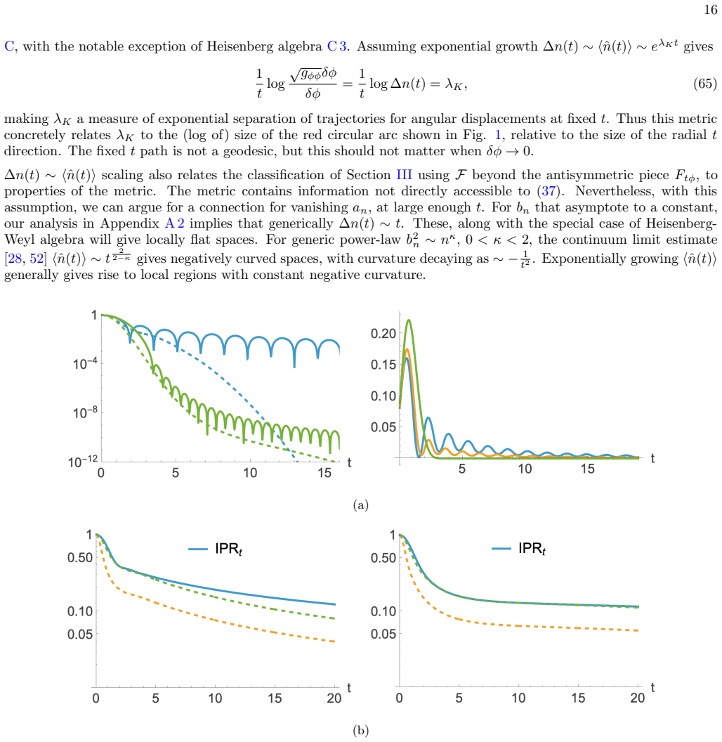
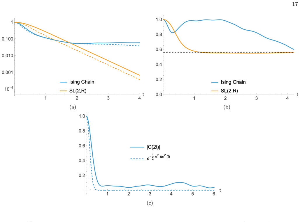
- Section IV, Eqs. (60)–(64): the exponentiated bound |G(t,φ)|≳exp(-1/2(Δn(t))²φ²) and the consequent IPR estimates are presented as physically motivated but non-rigorous. They fail near zeros of C(2t) and are only verified numerically on selected models. Because they are used to constrain the complexity distribution, the manuscript should either (i) state clearly that they are heuristic estimates outside the rigorous core, or (ii) supply a controlled error estimate (e.g., after the proposed time-smearing) that quantifies the domain of validity.
- Section III.B and Appendix A.2: the late-time asymptotic for all moments under constant Lanczos coefficients (Eqs. 44, A19) relies on a factorized low-frequency ansatz for ñ(E,ω). While the leading power is checked numerically for k=1–3,6, a sharper statement of the error incurred by discarding the mean-energy dependence of A2(E) would strengthen the claim that the entire distribution is obtained from the spectral function alone.
minor comments (5)
- Figure 1 caption and surrounding text: the visual guide is helpful, but the right-hand panel (τ-rotation of the Krylov basis) is only sketched; a short explicit formula linking B(τ) to the Toda flow would improve readability.
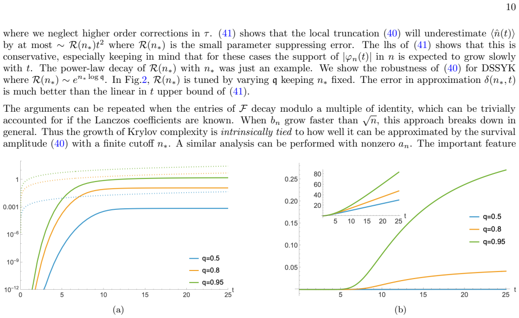
- Eq. (41) and Fig. 2: the truncation error bound is stated for a_n=0; a one-sentence remark on the nonzero-a_n case (already mentioned later) would avoid ambiguity.
- Appendix B, Eq. (B3): the approximate kernel is central to the late-time claims; a brief numerical comparison of the integrated moments against exact φ_n(t) for a non-constant bounded Φ(E) would make the accuracy claim more concrete.
- Notation: the same letter K is used for the Poisson kernel and, occasionally, for Krylov complexity; a consistent distinction (e.g., K vs. ⟨n̂⟩) would reduce minor confusion.
- References: the recent reviews [2,3] and the adiabatic-gauge-potential literature [25,43] are appropriately cited; a pointer to the original Loschmidt-echo Lyapunov papers [21–23] already appears, but a short sentence linking the present nonlocal φ-deformation to those semiclassical results would help non-specialist readers.
Circularity Check
No significant circularity: central identities follow by construction from the Krylov algebra and Fubini-Study metric without fitted parameters or load-bearing self-citation.
full rationale
The paper's strongest claims are algebraic identities, not empirical predictions. Krylov complexity is defined as the mean of the number operator n̂ on the Krylov chain (Eq. 17). The commutation relations [n̂, L±] = ±L± (Eq. 20) immediately imply the Heisenberg evolution M(ϕ) = e^{i n̂ ϕ} M e^{-i n̂ ϕ} (Eq. 23). Differentiating the resulting Loschmidt amplitude G(t, ϕ) = ⟨0|e^{i M t} e^{-i M(ϕ) t}|0⟩ with respect to ϕ at ϕ = 0 recovers ⟨n̂(t)⟩ by definition (Eqs. 24a–26). The volume bound ⟨n̂(t)⟩ ≤ (1/π) Vol_t (Eq. 54) is likewise an immediate consequence of the Robertson–Schrödinger uncertainty relation applied to the Fubini–Study metric components (Eqs. 51–53); equality holds precisely when the complexity algebra closes, which is verified by direct computation in Appendix C rather than assumed. The spectral-propagator representation (Eq. 27) and the τ-deformation that yields ∂t ⟨n̂⟩ (Eq. 37) are likewise rearrangements of the same operators. Model checks (DSSYK Lanczos sequence (D4), SL(2,R) coherent states (C20), constant-b RMT) use previously published sequences without re-fitting any free parameter to the complexity data being “predicted.” The only non-rigorous statements—the exponentiated bound |G| ≳ exp(−½(Δn)^{2} ϕ^{2}) (Eq. 60) and the consequent IPR estimates (Eqs. 63–64)—are explicitly labeled as physically motivated hypotheses and are not used to derive the two central claims. No uniqueness theorem is imported from the author’s prior work, no ansatz is smuggled via self-citation, and no fitted input is renamed a prediction. The derivation chain is therefore self-contained and non-circular.
Axiom & Free-Parameter Ledger
axioms (4)
- standard math The Krylov number operator satisfies [n̂,L±]=±L± and B=i[n̂,M] is the conjugate momentum (Eqs. 20–21).
- standard math The Fubini-Study metric on the projective Hilbert space induces a Riemannian metric on any smooth submanifold of states (Eqs. 48–49).
- domain assumption For spectral densities supported on a finite interval the orthonormal polynomials admit the Szegő asymptotics (B1)–(B2).
- standard math When the Frobenius norm of F is finite, Cauchy–Schwarz yields the complexity bound (47).
invented entities (2)
-
Spectral propagator (Poisson kernel) K(E1,E2,ϕ)
no independent evidence
-
Complexity geometry (t,ϕ) with metric components (51)
no independent evidence
read the original abstract
Krylov complexity is a powerful diagnostic of quantum dynamics, with clear connections to other measures of quantum chaos and operator growth. One such measure is the Loschmidt amplitude, defined as the overlap of initially identical states evolved under two slightly different Hamiltonians. Its decay in certain systems is controlled by the classical Lyapunov exponent. Using the algebraic properties of the Krylov complexity operator, we express Krylov complexity as the derivative of a Loschmidt amplitude whose perturbation is parameterized by an angular variable $\phi$. This formulation allows us to define a spectral propagator that encodes the entire complexity distribution, which we characterize for specific types of systems. We study the two-dimensional quantum geometry spanned by time and $\phi$ where the original and deformed trajectories reside, demonstrating that Krylov complexity is upper-bounded by its volume. We also express the time derivative of Krylov complexity in terms of a distinct Loschmidt amplitude. Depending on the growth of the Lanczos coefficients, the perturbation term in this amplitude can be truncated. We propose that the strength of this perturbation provides a classification scheme for Krylov complexity dynamics and relate it to the $\phi$-derivative of the spectral propagator. Using this analytical framework, we derive general relations between the time-dependence of the survival amplitude and Krylov space measures.
Figures


Reference graph
Works this paper leans on
-
[1]
Just the 11 existence of|| F ||constrains the asymptotic growth of complexity through (43), as shown below in (47) and through the analysis of the kernel in Appendix A 3
Since the Frobenius norm is unitarily invariant:|| ˜F ||=|| F ||, whenever well-defined, it provides a sum-rule for the matrix elements ˜F jk. Just the 11 existence of|| F ||constrains the asymptotic growth of complexity through (43), as shown below in (47) and through the analysis of the kernel in Appendix A 3. Whenever Φ(E) is bounded i.e Φ(E) = 0 for|E...
-
[2]
As long as the measure is even, meaning thata n continue to vanish,g tϕ = 0 and the metric is diagonal
obtained the two-dimensional maximally symmetric spaces of constant curvature in the case of operator complex- ity, where all thea n vanish. As long as the measure is even, meaning thata n continue to vanish,g tϕ = 0 and the metric is diagonal. From (28),(21), combined with theϕisometry, it simply follows thatF ϕt is the time derivative of Krylov complexi...
-
[3]
Krylov- winding
TheSL(2, R) toy model (orange) is specified by the Lanczos coefficients (C20), where both theb n anda n coefficients have been perturbed by independent positive random variables with mean 0.25. For theSL(2, R) computationα= 1, γ= 0.1, h= 1 2.(c) Illustration of (61)in spin chain:Ising chain with same parameters and initial operator as above used. This amp...
2024
-
[4]
D. E. Parker, X. Cao, A. Avdoshkin, T. Scaffidi, and E. Altman, A universal operator growth hypothesis, Physical Review X9, 10.1103/physrevx.9.041017 (2019)
-
[5]
E. Rabinovici, A. S´ anchez-Garrido, R. Shir, and J. Sonner, Krylov complexity (2025), arXiv:2507.06286 [hep-th]
Pith/arXiv arXiv 2025
-
[6]
Nandy, A
P. Nandy, A. S. Matsoukas-Roubeas, P. Mart´ ınez-Azcona, A. Dymarsky, and A. del Campo, Quantum dynamics in krylov space: Methods and applications, Physics Reports1125-1128, 1–82 (2025)
2025
-
[8]
S.-K. Jian, B. Swingle, and Z.-Y. Xian, Complexity growth of operators in the syk model and in jt gravity, Journal of High Energy Physics2021, 10.1007/jhep03(2021)014 (2021)
-
[9]
P. Caputa and S. Datta, Operator growth in 2d cft, Journal of High Energy Physics2021, 10.1007/jhep12(2021)188 (2021)
-
[10]
A. Kar, L. Lamprou, M. Rozali, and J. Sully, Random matrix theory for complexity growth and black hole interiors, Journal of High Energy Physics2022, 10.1007/jhep01(2022)016 (2022)
-
[11]
J. Kim, J. Murugan, J. Olle, and D. Rosa, Operator delocalization in quantum networks, Physical Review A105, 10.1103/physreva.105.l010201 (2022)
-
[12]
M. Alishahiha and S. Banerjee, A universal approach to krylov state and operator complexities, SciPost Physics15, 10.21468/scipostphys.15.3.080 (2023)
-
[13]
P. Caputa, N. Gupta, S. S. Haque, S. Liu, J. Murugan, and H. J. R. Van Zyl, Spread complexity and topological transitions in the kitaev chain, Journal of High Energy Physics2023, 10.1007/jhep01(2023)120 (2023). 19
-
[14]
J. Erdmenger, S.-K. Jian, and Z.-Y. Xian, Universal chaotic dynamics from krylov space, Journal of High Energy Physics 2023, 10.1007/jhep08(2023)176 (2023)
-
[15]
M. P. Heller, J. Papalini, and T. Schuhmann, Krylov spread complexity as holographic complexity beyond jackiw-teitelboim gravity, Physical Review Letters135, 10.1103/spcr-jgm6 (2025)
-
[16]
P. Nandy, T. Pathak, Z.-Y. Xian, and J. Erdmenger, Krylov space approach to singular value decomposition in non- hermitian systems, Physical Review B111, 10.1103/physrevb.111.064203 (2025)
-
[17]
S. E. Aguilar-Gutierrez, H. A. Camargo, V. Jahnke, K.-Y. Kim, and M. Nishida, Krylov operator complexity in holographic cfts: Smeared boundary reconstruction and the dual proper radial momentum, Physical Review D112, 10.1103/6bgg-vglp (2025)
-
[18]
I. Ermakov and O. Lychkovskiy, Symbolic recursion method for strongly correlated fermions in two and three dimensions (2026), arXiv:2512.23678 [cond-mat.str-el]
arXiv 2026
-
[19]
J. Maldacena, S. H. Shenker, and D. Stanford, A bound on chaos, Journal of High Energy Physics2016, 10.1007/jhep08(2016)106 (2016)
-
[20]
V. Balasubramanian, P. Caputa, J. M. Magan, and Q. Wu, Quantum chaos and the complexity of spread of states, Physical Review D106, 10.1103/physrevd.106.046007 (2022)
-
[21]
Peres, Stability of quantum motion in chaotic and regular systems, Phys
A. Peres, Stability of quantum motion in chaotic and regular systems, Phys. Rev. A30, 1610 (1984)
1984
-
[22]
Wisniacki, Loschmidt echo, Scholarpedia7, 11687 (2012)
A. Wisniacki, Loschmidt echo, Scholarpedia7, 11687 (2012)
2012
-
[23]
Gorin, T
T. Gorin, T. Prosen, T. H. Seligman, and M. ˇZnidariˇ c, Dynamics of loschmidt echoes and fidelity decay, Physics Reports 435, 33–156 (2006)
2006
-
[24]
R. A. Jalabert and H. M. Pastawski, Environment-independent decoherence rate in classically chaotic systems, Physical Review Letters86, 2490–2493 (2001)
2001
-
[25]
P. Jacquod, P. Silvestrov, and C. Beenakker, Golden rule decay versus lyapunov decay of the quantum loschmidt echo, Physical Review E64, 10.1103/physreve.64.055203 (2001)
-
[26]
P. Jacquod, I. Adagideli, and C. W. J. Beenakker, Decay of the loschmidt echo for quantum states with sub-planck-scale structures, Physical Review Letters89, 10.1103/physrevlett.89.154103 (2002)
-
[28]
M. Pandey, P. W. Claeys, D. K. Campbell, A. Polkovnikov, and D. Sels, Adiabatic eigenstate deformations as a sensitive probe for quantum chaos, Physical Review X10, 10.1103/physrevx.10.041017 (2020)
-
[29]
Szeg¨ o,Orthogonal Polynomials, Vol
G. Szeg¨ o,Orthogonal Polynomials, Vol. 23 (American Mathematical Society, Providence, RI, 1959)
1959
-
[30]
P. Caputa, J. M. Magan, and D. Patramanis, Geometry of Krylov complexity, Phys. Rev. Res.4, 013041 (2022), arXiv:2109.03824 [hep-th]
Pith/arXiv arXiv 2022
-
[31]
M¨ uck and Y
W. M¨ uck and Y. Yang, Krylov complexity and orthogonal polynomials, Nuclear Physics B984, 115948 (2022)
2022
-
[32]
J. Murugan and H. J. R. van Zyl, A Schwinger-Keldysh Formulation of Semiclassical Operator Dynamics (2026), arXiv:2602.02106 [quant-ph]
arXiv 2026
-
[33]
B. Bhattacharjee, P. Nandy, and T. Pathak, Krylov complexity in large q and double-scaled syk model, Journal of High Energy Physics2023, 10.1007/jhep08(2023)099 (2023)
-
[34]
D. Chakraborty and D. Rosa, Revival Dynamics from Equilibrium States: Scars from Chords in SYK (2025), arXiv:2512.16836 [cond-mat.str-el]
arXiv 2025
-
[35]
H. W. Lin, The bulk hilbert space of double scaled syk, Journal of High Energy Physics2022, 10.1007/jhep11(2022)060 (2022)
-
[36]
E. Rabinovici, A. S´ anchez-Garrido, R. Shir, and J. Sonner, A bulk manifestation of Krylov complexity, JHEP08, 213, arXiv:2305.04355 [hep-th]
-
[37]
J. Xu, On chord dynamics and complexity growth in double-scaled SYK, JHEP06, 259, arXiv:2411.04251 [hep-th]
-
[38]
S. E. Aguilar-Gutierrez, Building the holographic dictionary of the DSSYK from chords, complexity & wormholes with matter, JHEP10, 221, arXiv:2505.22716 [hep-th]
-
[39]
P. Bueno, J. M. Magan, and C. S. Shahbazi, Complexity measures in QFT and constrained geometric actions, JHEP09, 200, arXiv:1908.03577 [hep-th]
Pith/arXiv arXiv 1908
-
[40]
H. W. Lin and L. Susskind, Complexity geometry and schwarzian dynamics, Journal of High Energy Physics2020, 10.1007/jhep01(2020)087 (2020)
-
[41]
V. Balasubramanian, P. Caputa, and J. Sim´ on, Variations on a theme of krylov (2025), arXiv:2511.03775 [hep-th]
arXiv 2025
-
[42]
N. Angelinos, D. Chakraborty, and A. Dymarsky, Temperature dependence in Krylov space, J. Phys. A59, 235204 (2026), arXiv:2508.19233 [hep-th]
Pith/arXiv arXiv 2026
-
[43]
E. Rabinovici, A. S´ anchez-Garrido, R. Shir, and J. Sonner, Operator complexity: a journey to the edge of krylov space, Journal of High Energy Physics2021, 10.1007/jhep06(2021)062 (2021)
-
[44]
V. Balasubramanian, J. M. Magan, and Q. Wu, Quantum chaos, integrability, and late times in the Krylov basis, Phys. Rev. E111, 014218 (2025), arXiv:2312.03848 [hep-th]
Pith/arXiv arXiv 2025
-
[45]
Chakraborty,Topics in Quantum Information, Complexity and Chaos, Ph.D
D. Chakraborty,Topics in Quantum Information, Complexity and Chaos, Ph.D. thesis, University of Kentucky (2024)
2024
-
[46]
Kolodrubetz, D
M. Kolodrubetz, D. Sels, P. Mehta, and A. Polkovnikov, Geometry and non-adiabatic response in quantum and classical systems, Physics Reports697, 1–87 (2017)
2017
-
[47]
Caputa, B
P. Caputa, B. Chen, R. W. McDonald, J. Sim´ on, and B. Strittmatter, Spread complexity rate as proper momentum, Phys. Rev. D113, L041901 (2026)
2026
-
[48]
M. V. Berry, Quantal phase factors accompanying adiabatic changes, Proc. Roy. Soc. Lond. A392, 45 (1984). 20
1984
-
[49]
D. J. Thouless, M. Kohmoto, M. P. Nightingale, and M. den Nijs, Quantized hall conductance in a two-dimensional periodic potential, Phys. Rev. Lett.49, 405 (1982)
1982
-
[50]
Simon, Holonomy, the quantum adiabatic theorem, and berry’s phase, Phys
B. Simon, Holonomy, the quantum adiabatic theorem, and berry’s phase, Phys. Rev. Lett.51, 2167 (1983)
1983
-
[51]
X.-L. Qi, Y.-S. Wu, and S.-C. Zhang, Topological quantization of the spin hall effect in two-dimensional paramagnetic semiconductors, Physical Review B74, 10.1103/physrevb.74.085308 (2006)
-
[52]
N. H¨ ornedal, N. Carabba, A. S. Matsoukas-Roubeas, and A. del Campo, Ultimate speed limits to the growth of operator complexity, Communications Physics5, 10.1038/s42005-022-00985-1 (2022)
-
[53]
T. Ozawa and B. Mera, Relations between topology and the quantum metric for chern insulators, Physical Review B104, 10.1103/physrevb.104.045103 (2021)
-
[54]
Perugu, B
R. Perugu, B. Kobrin, M. O. Flynn, and T. Scaffidi, Krylov winding and emergent coherence in operator growth dynamics, Phys. Rev. Lett.136, 150402 (2026)
2026
-
[55]
J. Barb´ on, E. Rabinovici, R. Shir, and R. Sinha, On the evolution of operator complexity beyond scrambling, Journal of High Energy Physics2019, 10.1007/jhep10(2019)264 (2019)
-
[56]
Deift, T
P. Deift, T. Kriecherbauer, K. T.-R. McLaughlin, S. Venakides, and X. Zhou, Strong asymptotics of orthogonal polynomials with respect to exponential weights, Communications on Pure and Applied Mathematics52, 1491 (1999)
1999
-
[57]
Deift, T
P. Deift, T. Kriecherbauer, K. T.-R. McLaughlin, S. Venakides, and X. Zhou, A riemann–hilbert approach to asymptotic questions for orthogonal polynomials, Journal of Computational and Applied Mathematics133, 47 (2001)
2001
-
[58]
Ismail,Interplay Between Computational Techniques and Quantum Theory: Advancing Quantum Chaos and Quantum Error Correction, Ph.D
R. Ismail,Interplay Between Computational Techniques and Quantum Theory: Advancing Quantum Chaos and Quantum Error Correction, Ph.D. thesis, Kentucky University (2025)
2025
-
[59]
R. Basu, P. Chowdhury, A. Ganguly, S. Nath, O. Parrikar, and S. Paul, Wigner negativity, random matrices and gravity, JHEP01, 106, arXiv:2506.02110 [hep-th]
-
[60]
R. Basu, A. Ganguly, S. Nath, and O. Parrikar, Complexity growth and the krylov-wigner function (2025), arXiv:2402.13694 [hep-th]
arXiv 2025
-
[61]
A. Avdoshkin and A. Dymarsky, Euclidean operator growth and quantum chaos, Physical Review Research2, 10.1103/phys- revresearch.2.043234 (2020). Appendix A: Poisson Kernel
doi:10.1103/phys- 2020
-
[62]
The Krylov basis is specified by orthogonal polynomials given in (12)
General Formalism In this section, having taken the thermodynamic limit first, we consider a continuous energy spectrum which makes the spectral function Φ(E) continuous and normalized it to be consistent with⟨0|0⟩= 1. The Krylov basis is specified by orthogonal polynomials given in (12). In terms of the orthonormal polynomialsp n(E), we define the Poisso...
-
[63]
The derivatives∂ k ϕK(E1, E2, ϕ) will typically only be distributional atϕ= 0
Modeling the kernels If we can directly estimateK(E 1, E2, ϕ) through exact results or asymptotics, then it may be advantageous to compute (27) though saddle point or numerical integration and then take derivatives. The derivatives∂ k ϕK(E1, E2, ϕ) will typically only be distributional atϕ= 0. They might only make sense through a regularization forr. It m...
-
[64]
The relevant integral which gives the square of the Frobenius norm is RR | ˜F(E 1, E2)|2dE1dE2
Frobenius Norm Constraint Now we consider a system where ˜F(E 1, E2) is square-integrable, despite the Lanczos coefficients growing without bound. The relevant integral which gives the square of the Frobenius norm is RR | ˜F(E 1, E2)|2dE1dE2. This can be checked by explicitly plugging in the definition (A8) in terms of matrix elements. Generically, in suc...
-
[65]
This matches the asymptotic growth rate predicted by (47), with the additional assumption that lim t→∞ C(t) = 0
The upper boundχ= 1 2 gives a late-time asymptotic oft 3 2 . This matches the asymptotic growth rate predicted by (47), with the additional assumption that lim t→∞ C(t) = 0. Appendix B: Asymptotics for spectral function with bounded support We now discuss asymptotics for orthogonal polynomials when the spectral function Φ(x) has support only on a finite s...
-
[66]
We restrict to the simple case whereMandBare exactly like the position and momentum operator
Heisenberg Algebra Here we consider the Heisenberg algebra familiar from the harmonic oscillator [a, a †] = 1. We restrict to the simple case whereMandBare exactly like the position and momentum operator. M=α a+a † , B=iα a† −a ,F= 2α 2I.(C38) The time-evolving state|ψ(t)⟩is a coherent state of the harmonic oscillator. This gives φn(t) =e −α2t2/2 αntn √ n...
-
[67]
Double-Scaled SYK The SYK model is specified by the disordered Hamiltonian H=i p 2 X 1<j1<j2<...<jp<N Jj1j2...jp ψj1 ψj2 . . . ψjp ,(D1) whereψ k denotes Majorana fermions at sitek, andJ j1,j2...jp is a Gaussian random variable specifying thepbody interaction with the ensemble averaged first and second moments Jj1j2...jp = 0 D J2 j1j2...jp E = 1 4 N p (D2...
-
[68]
forward” and “backward
Finite Ising spin chain For our numerics we used the finite-sized nonintegrable Ising spin chain with the parameters H=− i=6X i=1 σx i σx i+1 + 7X i=1 (0.8σx i + 1.05σz i ) (D6) in terms of the Pauli matricesσ α i at the sitei. The Krylov space dimension isN= 16257. Appendix E: Refined Dyck Paths Here we will describe a combinatorial method for evaluating...
discussion (0)
Sign in with ORCID, Apple, or X to comment. Anyone can read and Pith papers without signing in.