Data Field Theory: Theory and Applications of the Functional Renormalization Group for Signal Detection

Dine Ousmane Samary; Parham Radpay; Riccardo Finotello; Vincent Lahoche

REVIEW 5 major objections 5 minor 14 references

A signal buried in the noise bulk can be found by watching the effective dimension of a data field theory run with scale.

Reviewed by Pith at T0; open to challenge. T0 means a machine referee read the full paper against a public rubric. the ladder, T0–T4 →

Challenge this review Re-run · record.json Download PDF Read on arXiv ↗

T0 review · deepseek-v4-flash

2026-08-01 04:24 UTC pith:7LRUY7K4

load-bearing objection A well-written review of the authors' own FRG detection program, with internally consistent math and a promising Ising benchmark — but the headline LOD claim compares against the wrong baseline, and the detection criterion reduces to an edge-exponent test. the 5 major comments →

arxiv 2607.27236 v1 pith:7LRUY7K4 submitted 2026-07-24 physics.data-an cond-mat.stat-mechcs.ITmath.ITstat.ME

Data Field Theory: Theory and Applications of the Functional Renormalization Group for Signal Detection

Riccardo Finotello , Vincent Lahoche , Dine Ousmane Samary , Parham Radpay This is my paper

classification physics.data-an cond-mat.stat-mechcs.ITmath.ITstat.ME

keywords renormalization groupfunctional renormalization groupdata field theoryrandom matrix theorysignal detectiondimensional phase transitionspectral tailextensive-rank signals

verification ladder T0 review T1 audit T2 compute T3 formal T4 reserved

The pith

A machine-rendered reading of the paper's core claim, the machinery that carries it, and where it could break.

This review argues that signal detection in high-dimensional data can be reformulated as a renormalization-group question: build an effective field theory whose two-point function reproduces the empirical covariance spectrum, then ask whether the Gaussian fixed point of the pure-noise universality class is stable under coarse-graining. The central claim is that a signal of extensive rank—one that does not separate from the noise bulk as isolated spikes—deforms the spectral tail and makes the canonical dimensions of interactions run with scale. When the running dimension of the quartic coupling crosses zero at effective dimension four, the flow switches from non-Gaussian noise to Gaussian-dominated signal behaviour, giving an objective scale at which to cut the spectrum. In synthetic-image tests the method flags signals at strengths roughly six times below the classical spike-detection threshold, and it recovers the exact critical temperature of a two-dimensional spin-lattice model to about two percent. Because only the eigenvalue distribution enters, the same logic transfers across datasets, from images to financial correlations to sensor arrays.

Core claim

The paper's central claim is that the presence of a signal in a high-dimensional dataset reveals itself as a dimensional phase transition in an effective field theory built from the empirical correlation spectrum. Pure noise belongs to a universality class whose spectrum has a square-root edge and whose effective field theory behaves like a three-dimensional theory with a relevant quartic coupling; the Gaussian fixed point is unstable. A signal of extensive rank deforms the tail of the spectrum, changing the effective momentum-space measure ρ(p²), and thereby making the canonical dimension of the quartic coupling scale-dependent. The scale at which dimτ(u4)=0 marks the upper critical dimensi

What carries the argument

The central object is the data field theory: an effective field theory whose Gaussian two-point function is fixed to reproduce the empirical correlation matrix, with the eigenvalue density serving as the momentum-space measure. The load-bearing mechanism is the scale-dependent canonical dimension of the quartic coupling, computed from the functional renormalization-group flow of a local, Z2-symmetric effective potential truncated at order u6. Because the empirical spectral measure is not a power law, the canonical dimension is not constant; it runs with scale, and the condition dimτ(u4)=0 defines the dimensional phase transition at effective dimension D=4. The flow equations, solved in the l

Load-bearing premise

The load-bearing premise is that the deformed spectrum can be faithfully summarized by a simple, symmetric field theory with only quartic and sextic interactions; if real signal-induced correlations require non-local or higher-order couplings at the detection scale, the criterion would read pure noise and miss the signal.

What would settle it

Run the numerical flow for the same empirical spectrum from two different ultraviolet starting scales (for example, k²=10 and k²=20) and compare the canonical dimensions at the infrared scale k_IR; if they differ materially, the paper's assertion that canonical dimensions are independent of the prior flow history fails, and the plotted dimτ values are not well-defined functions of the spectrum.

Watch this falsifier — get emailed when new claim-graph text bears on it.

If this is right

A lower limit of detection: in the synthetic test, the framework flags signals at strength roughly 0.15, while the classical spike-separation threshold sits near 0.97—about six times higher.
An objective cutoff: the scale where the quartic coupling dimension vanishes replaces an arbitrary eigenvalue cutoff, so the signal/noise boundary follows from the spectrum itself rather than a user-chosen threshold.
Universality transfer: since only the eigenvalue distribution enters, a detector calibrated on one noise source in the universal class applies to any other dataset in the same class, whatever the microscopic origin.
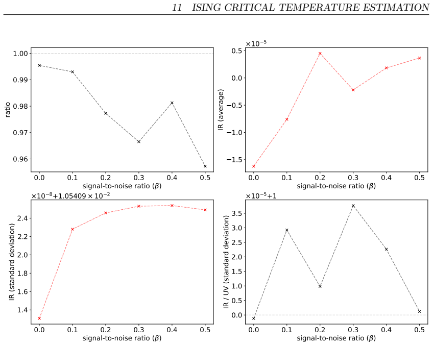
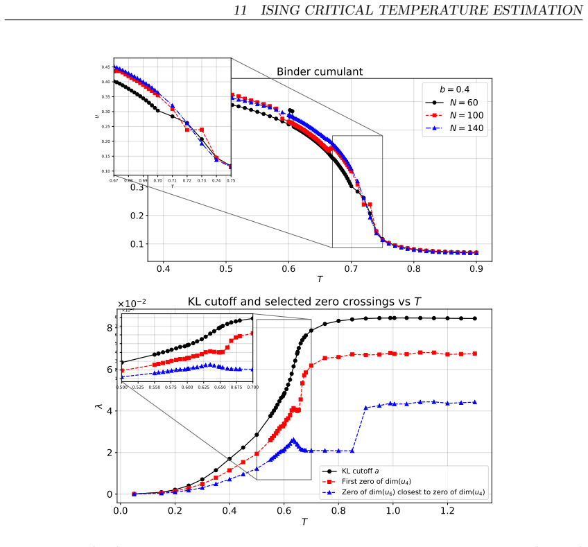
Physical benchmark: the dimensional criterion recovers the exact critical temperature of the two-dimensional spin-lattice model to about 2%, outperforming divergence-minimization baselines at about 7% error.
A second signature: at the transition the eigenvector statistics change from delocalized Gaussian toward localized, giving an independent cross-check of the detection thresholds.

Where Pith is reading between the lines

These are editorial extensions of the paper, not claims the author makes directly.

If the paper's asserted history-independence of canonical dimensions can be proven, canonical dimensions become a well-defined spectral statistic, potentially making the detector fully parameter-free and independent of the integration scheme.
The framework suggests a reinterpretation of denoising: instead of deleting eigenvalues beyond a cutoff, one could project out the flow directions that leave the basin of the Gaussian fixed point, preserving collective signal deformations.
A natural stress test is to apply the criterion to spectra with known non-local correlations, such as block-structured covariance with weak off-diagonal weights; if the quartic-dimension crossing still tracks signal strength, the locality assumption is broader than feared, and if not, the universality claim needs qualification.
The numerical thresholds could be compared against the finite-size fluctuation scale P^{-2/3} to derive an analytic expression for the limit of detection as a function of sample size and aspect ratio.

Editorial analysis

A structured set of objections, weighed in public.

Desk editor's note, referee report, simulated authors' rebuttal, and a circularity audit.

Desk Editor's Note

A well-written review of the authors' own FRG detection program, with internally consistent math and a promising Ising benchmark — but the headline LOD claim compares against the wrong baseline, and the detection criterion reduces to an edge-exponent test.

read the letter

Two things to know. First, this is exactly what it says on the tin: a review of the authors' own FRG signal-detection program, drawing on [8–14], so don't expect new results; the novelty is in the pedagogical repackaging and one new proof-of-concept benchmark. Second, the headline claim — that the RG approach consistently yields a lower limit of detection than BBP — is not supported by the evidence in the paper, because the comparison is against a method the paper itself rules out for the target regime. That doesn't sink the program, but it does mean the central comparative claim needs work.

What's good: Part I is a genuinely clear RG primer for non-physicists. The flow equations (9.13–9.16) are internally consistent, and the zero-signal curves match the analytic MP predictions in Fig. 10.4. The intrinsic-variability analysis is careful: β0 ≈ 1.5e-3 vs βt ≈ 0.15 is a clean separation of scales. And the 2D Ising benchmark recovering Onsager within ~2% is a real external test, assuming the binning/pruning/IR-cutoff constants weren't tuned to it — the truncated §11.2 doesn't fully establish that, but it's a promising result. The authors also honestly catalog their approximation limits: the learnable region, the regulator bound, the scale-dependence of 'signal'.

Soft spots, in order of seriousness. (1) The comparative LOD claim is an apples-to-oranges comparison. β_BBP = q^{1/4} is the threshold for a single finite-rank spike (Appendix F), which the paper explicitly excludes as the target regime (Remark 10.2). No bulk-spectrum detector—KS or AD test against MP, residual-bulk largest-eigenvalue test, direct edge-exponent estimator—is benchmarked. Without those, "lower LOD than BBP" is beside the point. (2) The stress-test observation is correct: by the paper's own equations, dimτ(u4)=0 is exactly the condition that the spectral edge exponent α crosses 1 (Eq. 10.10, Def. 9.1, Eq. 9.69). The "dimensional phase transition" is a relabeling of an edge-exponent test. That doesn't make the RG machinery useless, but it does mean the paper needs to show what the RG buys you over a simpler edge-exponent estimate. (3) The locality/truncation of the EFT is assumed, not derived—collapsing the four-point tensor to δ_ij δ_kl δ_il and enforcing momentum conservation is a big reduction, and the paper's justification ("standard observation from the ordinary Fourier transform") doesn't address whether signal-induced non-localities matter. (4) The claim that canonical dimensions are independent of prior RG flow history (§10.2) is asserted without proof. That's load-bearing and should be proven or removed.

Who's it for: physicists and data scientists who want a self-contained entry into the FRG approach to spectral analysis. The review is well-written and honest about its limitations, but the comparative advantage claim is overreach. It deserves a serious referee; I'd send it back with a request for bulk-spectrum baselines, a direct statement of the edge-exponent equivalence, and a proof or caveat on the history-independence claim.

Referee Report

5 major / 5 minor

Summary. The paper reviews and develops Data Field Theory (DFT), a functional-renormalization-group framework for signal detection in high-dimensional data. The construction begins from an effective field theory whose propagator reproduces the empirical correlation spectrum, defines a generalized momentum variable, and derives dimensionless RG flow equations for the couplings u2, u4, u6 under the local potential approximation (Eqs. 9.13–9.16). The central claim is that a signal of extensive rank deforms the spectral tail, making the canonical dimensions scale-dependent and driving a 'dimensional phase transition' at effective dimension D0=4, at which the quartic coupling becomes irrelevant (Eq. 10.10). This is presented as yielding a lower limit of detection than the BBP threshold, with support from synthetic-image experiments (βt≈0.15 vs β_BBP≈0.97), eigenvector statistics, an Ising critical-temperature benchmark, and real-world hyperspectral data. The numerical implementation is stated to be available in a public GitHub library.

Significance. If the framework holds up, it addresses an important detection regime: signals that do not separate from the bulk as isolated spikes but instead deform the quasi-continuous spectrum. The paper has genuine strengths: the flow equations are internally consistent; the zero-signal canonical dimensions match the analytic MP predictions (Fig. 10.4); the intrinsic-variability analysis (β0≈1.5e-3 << βt, §10.4) supports statistical robustness; and the 2D Ising benchmark provides an independent physical check with reported accuracy near Onsager's value. The availability of reproducible numerical code is also a positive feature. However, the headline comparative claim against BBP is not yet established, because the comparison target is a spike-detection threshold, not a bulk-spectrum detector. The detection criterion itself is shown to be equivalent to a local spectral-edge-exponent condition, so the paper must demonstrate that the RG machinery adds value over simpler spectral statistics.

major comments (5)

[§1, §10.3, Table 10.1, Fig. 10.4] The central comparison βt≈0.15 vs β_BBP≈0.97 is not probative. Appendix F defines β_BBP=q^{1/4} for a single finite-rank spike, and Remark 10.2 explicitly excludes that regime as the target of this framework. Since the paper addresses extensive-rank, bulk-deforming signals, the appropriate benchmarks are detectors designed for bulk spectral deformation: e.g., Kolmogorov–Smirnov or Anderson–Darling tests against the MP distribution, a largest-eigenvalue-of-residual-bulk statistic, or a direct edge-exponent estimator. Without such baselines, the abstract claim that the RG approach 'consistently yields a lower limit of detection than the BBP threshold' is unsupported.
[§9.4, Definition 9.1, Eqs. (9.69), (10.10)] The threshold βc is fixed by dimτ(u4)=0. By Eq. (9.69) and Definition 9.1, this is exactly the condition that the local spectral edge exponent α equals 1, i.e. D0=4. Thus the 'dimensional phase transition' is a reparametrization of a local edge-exponent condition. The paper should either test the RG criterion against direct estimates of α on the same synthetic datasets, or explicitly present the equivalence as the operational content of the method. The concern raised by the reader is therefore not strict circularity, but the criterion must be shown to outperform—or at least match—a simpler spectral statistic before the methodological novelty is established.
[§10.2] The statement 'It can be shown that the canonical dimensions are independent of the prior RG flow history' is load-bearing: the empirical plots of dimτ(u2), dimτ(u4), dimτ(u6) presuppose that these quantities are well-defined functions of the spectrum alone. No proof or reference is provided. If this claim fails, the entire detection observable is not uniquely defined. Please provide a derivation or a numerical check on the flow equations showing that integrating from different initial conditions yields the same canonical dimensions at a given k2.
[§7.3.2, Eqs. (7.19), (7.21), (7.24)] The local Z2-symmetric, momentum-conserving truncation is presented as forced by universality and as 'a standard observation from the ordinary Fourier transform.' But the empirical eigenbasis is not translation invariant, and the construction of a doubled momentum space with δ(Σ p_i) is an additional modeling assumption. If signal-induced spectral deformations generate non-local couplings, or if couplings beyond u6 become relevant at the detection scale, the criterion will not read the same. The authors should test the robustness of the detection thresholds against non-local or higher-order truncations on the same data, or clearly state this as a scope limitation.
[§11.2] The Ising benchmark is a genuine external validation, but the reported 2–3% agreement with Onsager's Tc and the comparison with KL-divergence minimization need more methodological detail: how the GSA cutoff is converted into a critical-temperature estimate, what error bars are used, and how the KL baseline is constructed. Without this detail, the benchmark cannot be independently assessed or replicated from the text alone.

minor comments (5)

[Definition 1.1] Eq. (1.1) appears to be missing a division sign: C_ij should presumably be (C0)_ij / sqrt((C0)_ii (C0)_jj). Please correct the typography.
[Theorem 1.1] In Eq. (1.3), λ± = σ^2(1±√q)^2 is intended; the current rendering '(1±√q)2' is easy to misread as multiplication.
[Eq. (9.16)] The last term of the flow equation for u6 is printed as −108 ¯u3^6/(1+¯u2)^4; dimensionally it should presumably be ¯u6^2. Please check and correct.
[Eq. (10.7)] The definition k2_IR = (k2_* − k2_0.5)/2 is ambiguous as typeset. Please add parentheses or an explicit sentence clarifying the construction.
[§10.3] The extraction of βt from Figure 10.5 uses a moving average with window width Δβ_w, but no uncertainty or cross-validation is reported. A short discussion of how the threshold depends on the smoothing window would strengthen the claim.

Circularity Check

2 steps flagged

Partial circularity: the 'dimensional phase transition' is a relabeling of the edge-exponent condition, and the synthetic LOD is defined by its own detector's departure.

specific steps

renaming known result [§9.4 (Definition 9.1, Eq. 9.69), §10.3 (Eq. 10.10)]
"A direct calculation further yields: dimτ(u4) = (1−α)/(1+α) = (4−D0)/D0. ... The signal, in this language, is the deviation of the canonical dimension from its MP value, evaluated at the location where dimτ(u4)=0. ... dimτ(u4)|λc = 0."

Combining Definition 9.1 (D0 = 2α+2) with Eq. 9.69, the condition dimτ(u4)=0 is exactly equivalent to D0=4 and hence to α=1. Thus the 'dimensional phase transition' and the detection criterion Eq. 10.10 are, by the paper's own equations, a relabeling of a local spectral-edge exponent condition (α=1). The RG vocabulary ('effective dimension', 'canonical dimension') is constructed from the empirical spectrum ρ(p²); the transition criterion therefore reduces by construction to a property of the input spectral edge rather than being an independent first-principles prediction.
fitted input called prediction [Table 10.1, §10.3 (Fig. 10.4/10.5)]
"βt Limit of detection (LOD). The 'rigidity' threshold at which the canonical dimensions begin to depart from the noise baseline. ... The canonical dimension remains largely invariant for low values of β, undergoing a significant transition only upon reaching a threshold identified as the LOD βt (in this instance, βt≈0.15)."

The synthetic-image LOD is not established by comparison with ground-truth labels or a pre-registered decision rule; βt is defined as the point where the detector's own canonical dimensions depart from the noise baseline. The statement 'βt≈0.15 is the LOD' is therefore true by construction, and the headline comparison βt ≪ β_BBP inherits this definition. The Ising benchmark validates a different quantity (critical-temperature estimation), not the claimed synthetic-image limit of detection.

full rationale

The paper's field-theoretic construction is self-contained in the sense that it explicitly derives the flow equations and canonical dimensions from the empirical spectrum, and the Ising benchmark provides genuine external validation. However, the central 'dimensional phase transition' criterion is a direct rewriting of the spectral edge exponent: by Definition 9.1 and Eq. 9.69, dimτ(u4)=0 iff α=1 (D0=4). This is a concrete reduction by the paper's own equations, making the detection criterion a relabeling of an input-spectrum property. Separately, the synthetic LOD βt is defined as the point where the canonical dimensions depart from baseline, so the claim that the RG 'yields' this LOD is tautological without an independent detection benchmark. The comparison to β_BBP is also made against a spiked-model threshold in a regime the paper explicitly excludes, but that is a correctness/benchmarking concern rather than circularity. I also note §10.2 asserts without proof that 'canonical dimensions are independent of the prior RG flow history'; this is an omitted proof on which the well-definedness of the plotted dimensions depends, but it is not itself a circular step. Overall, the circularity is partial: the formalism has independent content (especially the Ising benchmark), but two load-bearing 'predictions' reduce to definitions/relabelings, warranting a score of 5.

Axiom & Free-Parameter Ledger

4 free parameters · 8 axioms · 1 invented entities

The predictive claims rest on the MP noise model, the identification of signal with spectral-tail deformation, and a chain of modeling postulates (locality, Z2 symmetry, momentum conservation in the doubled space, u8-truncation, flow-history independence) that are largely carried over from the authors' prior works [8–14] rather than re-derived here. Hand-set constants (binning exponent, pruning scale, IR scale, smoothing window) enter the reported thresholds. The Onsager benchmark is the main external anchor, provided those constants were not tuned to it.

free parameters (4)

IR evaluation scale k²_IR = midpoint of k²_0.5 and k²_* (Eq. 10.7)
Sets the scale at which canonical dimensions are quoted. The paper argues the exact choice is 'largely arbitrary' (Section 10.2), yet it directly determines the plotted threshold values and the quoted dim(u4) values.
Histogram bin-width exponent α in Δ_phys = P^{-α} = α = 0.5
Section 10.2: 'we set α=0.5, matching the theoretical arguments'. Co-determines the empirical momentum distribution ρ(p²) that feeds the canonical dimensions.
Spike-pruning spacing threshold Δ~_phys = P^{-0.8}
Section 10.2: the cutoff for discarding isolated spikes is 'empirically appropriate'; controls how much of the spectrum is retained for the bulk analysis.
Smoothing window for canonical-dimension curves = Δβ_w = 2×10^{-2}, step Δβ = 5×10^{-4}
Section 10.3: the reported thresholds βt, βc, βO are read from moving averages of noisy dimension curves; their values depend on these choices.

axioms (8)

standard math Marchenko–Pastur theorem as the noise model; weakly correlated large covariance spectra converge to μ_MP
Theorem 1.1; the noise reference against which all deviations ('signals') are measured.
domain assumption Signal presence is equivalent to spectral deformation away from the MP universality class
Core modeling step (Section 7.2). The paper acknowledges the definition of signal is 'fundamentally a matter of scale' (Remark 10.1), so 'signal' is not separable from 'structured noise of other origin' without a chosen reference.
domain assumption Eigenvectors of noise-class correlation matrices are Haar-uniform (Porter–Thomas components)
Invoked (Sections 7.3.1, 9.4) to justify the momentum-space picture and the local δ(p-conservation) form of interactions; empirically checked only at β=0.
ad hoc to paper The minimal interaction is local and Z2-symmetric with W_ijkl ∝ δ_ijδ_klδ_il
Eq. (7.19), Section 7.3.2: the P^4 four-point tensor is collapsed to one coupling on the basis of an Ising analogy and universality, not derived for arbitrary data.
ad hoc to paper The doubled-momentum-space construction with momentum conservation reproduces the eigenbasis RG flow
Eqs. (7.21), (7.24): asserted as 'not an additional assumption, but rather a standard observation from the ordinary Fourier transform' (Section 7.3.2). Valid for Haar eigenvectors; assumed otherwise.
ad hoc to paper Canonical dimensions are determined solely by the position within ρ(p²), independent of RG flow history
Section 10.2: 'It can be shown that the canonical dimensions are independent of the prior RG flow history' — asserted, deferred to prior works [8–14].
domain assumption LPA/vertex truncation at u8 = 0 is adequate in the IR region where detection is performed
Standard FRG approximation; the paper itself delimits its validity to the 'learnable region' below Λ0 (Section 9.5).
domain assumption In the 2D Ising benchmark, the ECM spectral heavy-tail crossover encodes T near Tc monotonically in the assumed way
Section 11: 'the spectrum of the ECM... begins to exhibit a heavy-tailed, power-law form as the transition temperature is approached'. The functional relation between spectral shape and temperature is used empirically, not derived.

invented entities (1)

Scale-dependent effective dimension D(k) (asymptotic dimension D0) no independent evidence
purpose: Detection criterion: the 'dimensional phase transition' at D=4 (dimτ(u4)=0) marks the signal/noise boundary
Definition 9.1: D0 = 2α+2, a functional of the empirical spectral edge exponent. It is computed from the same spectrum it classifies and has no falsifiable handle outside the paper; it is an organizing relabeling, not a new degree of freedom.

pith-pipeline@v1.3.0-alltime-deepseek · 55855 in / 27024 out tokens · 279916 ms · 2026-08-01T04:24:13.230518+00:00 · methodology

0 comments

read the original abstract

We review the renormalization group framework for signal detection in high-dimensional data, tailored to the regime where the signal may be of extensive rank and does not separate from the noise bulk as isolated spikes. The framework provides a conceptually simple criterion for distinguishing signal from noise within a quasi-continuous spectral region near a random-matrix universality class. This scenario lies beyond the reach of standard methods such as the Baik-Ben Arous-P\'ech\'e threshold, which requires eigenvalues to be cleanly separated from the bulk. The renormalization group approach, by contrast, directly tracks spectral deformations and consistently yields a lower limit of detection without relying on spike separation. We review results that identify the presence of a signal by testing the stability of the Gaussian fixed point of an effective field theory for the collective behaviour of the degrees of freedom in the spectral tail, where the signal resides. We also discuss how the scale dependence of the canonical dimension, induced by the signal, manifests as a dimensional phase transition.

Figures

Figures reproduced from arXiv: 2607.27236 by Dine Ousmane Samary, Parham Radpay, Riccardo Finotello, Vincent Lahoche.

**Figure 1.1.** Figure 1.1: A typical experimental spectrum {µ(λ)}, featuring a quasi-continuous bulk and a set of isolated spikes. The definition of ‘meaningful information’, and, specifically, the position of the cutoff Λcutoff, depends on the choice of the noise model. 1. A quasi-continuous bulk, where the typical spacing δ between the eigenvalues satisfies min(N, P) −1 < δ ≪ p min(N, P)−1 when the size N of the correlation matr… view at source ↗

**Figure 1.2.** Figure 1.2: Illustration of the convergence toward MP universal law. The histogram corresponds to the empirical spectrum of a white Wishart matrix with a sample size 4 × 104 and a ratio q = 0.5. The blue lines materialise the limit MP (µMP) law. Theorem 1.1: Marchenko–Pastur Distribution Let X be an N ×P random matrix with i.i.d. entries of variance σ 2 . As N, P → ∞ while keeping the ratio q def == P/N fixed, the e… view at source ↗

**Figure 1.3.** Figure 1.3: Illustration of the rg universality: many microscopic (ultraviolet, uv) theories describe the same long-distance physics in the sense that they become indistinguishable in the low-energy (infrared, ir) regime. The underlying philosophy of this article follows its predecessors. We shall consider an analogous field theory in the vicinity of universal noise, built on the hypothesis that it faithfully reprod… view at source ↗

**Figure 3.1.** Figure 3.1: A spin configuration on a 2-dimensional lattice, i.e. the 2D Ising model. S = +1 spins are represented by an upward-pointing arrow, and S = −1 spins by a downward-pointing arrow. where the Ising’s Hamiltonian is: HIsing[{Si}] def == −J X ⟨i,j⟩ SiSj + X ND i=1 SiBi (3.5) where J > 0 characterises the interaction between spins, T is the temperature of the system, Bi is the value of the external magnetic fi… view at source ↗

**Figure 4.1.** Figure 4.1: The construction of spin blocks: spins are averaged inside blocks (A, B, and C, for example), defining the block spin (ΦA, ΦB, ΦC ), and the interaction between spins is replaced by an effective interaction between blocks derived from the latter. 1. Group spins into blocks (e.g. 2 × 2 or 3 × 3 blocks in 2D). 2. Replace each block with a single ‘block spin’ (Φblock) representing the average orientation of… view at source ↗

**Figure 4.2.** Figure 4.2: (Left) The steps of the renormalization group form a trajectory in the parameter space S. (Right) The flow behavior in the vicinity of the critical surface S∞ ⊂ S. Small fluctuations at the block scale are eliminated at each step, yet systems at every stage are compared on the same lattice. Kadanoff’s approach thus changes the model’s resolution: at each step both the effective degrees of freedom and the… view at source ↗

**Figure 4.3.** Figure 4.3: Behaviour of the Landau potential for T > T0 (yellow curve) or for T < T0 (blue curve). The only stable solution is M = 0 when T > T0, while two non-zero stable solutions appear when T < T0, giving M ∼ ±(T0 − T) 1/2 , the zero solution becoming unstable (see [PITH_FULL_IMAGE:figures/full_fig_p022_4_3.png] view at source ↗

**Figure 5.1.** Figure 5.1: Illustration of the flow in the neighbourhood of the Gaussian point in dimension D ≤ 4: the flow converges toward a subspace spanned by essential and marginal interactions, the ‘renormalizable’ subspace SR. In the case where the flow converges toward a stable fixed point, it is called the ‘large river effect’. and here again, v¯ is exponentially suppressed in the ir when D > 4. The same would hold true f… view at source ↗

**Figure 5.2.** Figure 5.2: Behaviour of the rg in the vicinity of the Gaussian fixed point for ϵ > 0 (on left) and ϵ < 0 (on right). The red region corresponds to the Gaussian region. Arrows are oriented toward ir scales. We can diagonalise this matrix, and by calling θ1 and θ2 the opposite of its eigenvalues, and O the matrix of the change of basis, O−1MO = −θ1 0 0 −θ2 . (5.35) We can then define the couplings in the eigenbas… view at source ↗

**Figure 7.1.** Figure 7.1: Deep ir and deep uv details of the eigenvalue distribution (left) and of the momenta distribution (right). The analytic MP distribution is shown on top, some empirical distribution with sample size N = 2500 and ratio q = 0.9 at the bottom. The black line is the numerical interpolation used to construct the empirical inverse distribution. Imposing the constraint (7.6), the maximum entropy estimator takes… view at source ↗

**Figure 8.1.** Figure 8.1: Illustration of the rg map from uv physics described by the Hamiltonian H to long range physics described by the effective action Γ . The effective action, also known as the generating functional of 1-particle irreducible (1PI) diagrams in physics, physically corresponds to the classical action of the classical field M(x) def == ⟨Φ(x)⟩, (8.7) though one should rather speak here of a ‘classical Hamiltoni… view at source ↗

**Figure 8.2.** Figure 8.2: Typical behaviour of the cut-off Rℓ(ζ). model discussed in Part I). To explicitly construct this effective action, the frg modifies the Hamiltonian by adding a mass-like term ∆Hℓ[Φ]: H[Φ] → H[Φ] + 1 2 X ζ ϕ(ζ)Rℓ(ζ)ϕ(ζ) | {z } def ==∆Hℓ[Φ] . (8.11) The function Rℓ(ζ) freezes large-scale fluctuations (ζ > ℓ), which acquire a large mass, whereas the uv modes (ζ < ℓ) maintain a small mass and are integrated … view at source ↗

**Figure 9.1.** Figure 9.1: Behaviour of the canonical dimensions for the MP distribution with σ 2 = 1 and q = 0.9 (black dashed curve, see Theorem 1.1). As explained in Section 2 and as will be further discussed in Part III, the presence of a signal makes interactions ‘less relevant’, notably by lowering the values of the asymptotic canonical dimensions of the sextic and quartic couplings. This has a consequence on the behaviour o… view at source ↗

**Figure 9.2.** Figure 9.2: Symmetric phase restoration as a function of the dimension D0 in the thermodynamic limit. thermodynamic limit (at large scales). Thus, trajectories that end up in the symmetric phase when D0 < 4 end up in the non-symmetric phase when D0 > 4 ( [PITH_FULL_IMAGE:figures/full_fig_p063_9_2.png] view at source ↗

**Figure 9.3.** Figure 9.3: Flow behaviour and symmetry restoration for D0 < 4 (left) and D0 > 4 (right). The same trajectory, with initial conditions (−0.05, 0.1), ends up in the symmetric phase in the first case but not in the second. structural information. A concrete realisation is provided by the quartic matrix model with coupling γ: at the critical point γ = −1/12, the system undergoes a phase transition affecting the univers… view at source ↗

**Figure 10.1.** Figure 10.1: Samples extracted from the mnist dataset [59] and used for numerical evaluations. Remark 10.1: Scale of the Additive Noise Model As already pointed out in the introduction, it is worth emphasising that the definition of a ‘signal’ is fundamentally a matter of scale. Prior to any artificial corruption, the data intrinsically contain a certain level of noise. Consequently, (10.3) is strictly valid only … view at source ↗

**Figure 10.2.** Figure 10.2: Realistic scenario considered in the analysis: a photo of a (plush) cat with a non-trivial background. For simplicity, we consider a monochrome version. ‘energy step’ into the rg flow, corresponding to a physical scale difference: ∆phys = P −α, (10.5) where the parameter α ∈ [0.5, 1) can be determined by analysing the distance between isolated spikes and the bulk momentum distribution. In our numerical … view at source ↗

**Figure 10.3.** Figure 10.3: Empirical distribution corresponding to [PITH_FULL_IMAGE:figures/full_fig_p069_10_3.png] view at source ↗

**Figure 10.4.** Figure 10.4: Behaviour of the canonical dimensions of [PITH_FULL_IMAGE:figures/full_fig_p071_10_4.png] view at source ↗

**Figure 10.5.** Figure 10.5: The behaviour of the canonical dimension at the scale k 2 IR is presented as a function of β. Computations were performed with a step size of ∆β = 5 × 10−4 . Solid lines represent a moving average with a window width of ∆βw = 2 × 10−2 , while the raw experimental values are rendered with reduced opacity [PITH_FULL_IMAGE:figures/full_fig_p072_10_5.png] view at source ↗

**Figure 10.6.** Figure 10.6: Typical behaviour of the canonical dimension in the mnist set. of u4 at scale k 2 IR vanishes, signifying a local critical dimension of exactly 4 (in this example, βc ≈ 0.32). This defines the critical scale λc (in the eigenvalue spectrum), marking the boundary between signal and noise: dimτ(u4) [PITH_FULL_IMAGE:figures/full_fig_p073_10_6.png] view at source ↗

**Figure 10.7.** Figure 10.7: (Left) Behaviour of the canonical dimension based on the analytical MP law. (Right) Behaviour of the empirical canonical dimension in the IR with respect to q (N fixed). 0.0 0.2 0.4 0.6 0.8 1.0 variance ( 2 ) 0 1 2 3 4 5 6 7 canonical dimensions ×10 1 dim(u2) dim(u4) dim(u6) 0.0 0.2 0.4 0.6 0.8 1.0 variance ( 2 ) 0.0 0.5 1.0 1.5 2.0 2.5 3.0 canonical dimensions dim(u2) dim(u4) dim(u6) [PITH_FULL_IMAGE:… view at source ↗

**Figure 10.8.** Figure 10.8: (Left) Behaviour of the canonical dimension based on the analytical MP law. (Right) Empirical behaviour of the canonical dimension in the IR as a function of q (with fixed N). Note that for β > βO, the canonical dimensions exhibit a secondary increase before decreasing again. This implies that the quartic coupling may regain relevance before its canonical dimension becomes negative once more. While we e… view at source ↗

**Figure 10.9.** Figure 10.9: Empirical canonical dimension in the ir as a function of q for a fixed snr (β = 1.25) and constant sample size (N = 2 × 104 ), using the dataset [PITH_FULL_IMAGE:figures/full_fig_p076_10_9.png] view at source ↗

**Figure 10.10.** Figure 10.10: Distribution of eigenvector components at β = 0 (pure noise regime), shown for the 100 eigenvectors associated with the smallest eigenvalues (uv) and the 100 eigenvectors corresponding to the MP bulk scale (ir). We focus on a non-equilibrium field theory model for this analysis. Specifically, we work with Model A, which can be viewed as the non-equilibrium (time-dependent) counterpart of the ordinary … view at source ↗

**Figure 10.11.** Figure 10.11: uv and ir distributions of eigenvector components for different values of β. quenched in a low-temperature bath. When the bath temperature lies below the critical temperature Tc, nucleation associated with ageing effects drives the appearance of domains that grow slowly over time according to a characteristic scaling law L(t) ∼ t n , (11.1) where L(t) also represents the typical correlation length of … view at source ↗

**Figure 10.12.** Figure 10.12: Summary of the statistical properties characterising the eigenvector distributions: the ratio of the components at the origin, the mean value, the standard deviation of the ir components, and the ratio of the ir-to-uv standard deviations. whether the dynamics is conservative. For further details, the reader may consult the references cited above and the monograph [63]. At the moment of the transition, … view at source ↗

**Figure 11.1.** Figure 11.1: Illustration of the phase ordering kinetics for the Ising-like stochastic model (Model A) considered in this paper. The three top images represent the evolution following a quench from T = ∞ at t < 0 (first image on the left) to T = 0.5 Tc at t = 0. The next two images correspond respectively to time steps 3 × 103 and 3.9 × 104 of the evolution. From left to right, the three bottom images correspond to … view at source ↗

**Figure 11.2.** Figure 11.2: (Top left) Behaviour of the spectrum found by the KL-proxy for high temperature, T = 5. (Top right) Behaviour in the vicinity of the critical regime T = 0.648. (Bottom) Behaviour below the critical temperature T = 0.350 for b = 0.8. 11.2 Critical Temperature Estimation When approaching Tc from above, the spectrum of the ecm of the Ising model shows a deformation of the tail of the distribution, which b… view at source ↗

**Figure 11.3.** Figure 11.3: (Top) Behaviour of the Binder cumulant for different grid sizes with b = 0.4. (Bottom) Empirical behaviour of λc for different temperatures with different methods for b = 0.8. common method relies on the behaviour of the magnetic susceptibility, χ def == ∂M/∂B, using the notation established in Part I. This method has a major drawback: while the susceptibility exhibits a singularity for an infinite syst… view at source ↗

**Figure 11.4.** Figure 11.4: Comparison of the critical temperatures Tc(b) obtained by the various methods, for different values of b and N = 100. The final point at b ≈ 1.8, corresponding to the ‘Ising-like’ case, is in good agreement with Onsager’s temperature (≈ 0.57). The mean-field approximation obtained through the Hartree method is given by the green curve (see Appendix C). In this work, P represents the analytic momentum … view at source ↗

**Figure 11.5.** Figure 11.5: Position of λc as a function of T with different methods: dimτ(u4) (top left), dimτ(u6) (top right), and KL divergence (bottom). 11.2.2 Ising Model In this subsubsection, we analyse the phase transition of the pure Ising model, corresponding to the parametrisation in (11.13) as ε → ∞, using a Monte Carlo method with J = 1/4. We no longer describe the dynamics of a continuous field but rather that of dis… view at source ↗

**Figure 11.6.** Figure 11.6: (Top) Binder cumulant of the Ising model for different system sizes. (Bottom) Absolute magnetisation for the Ising model for various values of N. occurs around T = 0.58 ± 0.01, which is in good agreement with the theoretical prediction. This constitutes a stringent validation of gsa: the canonical dimension of the sextic coupling detects the Ising transition to within approximately 2% (the central value… view at source ↗

**Figure 12.1.** Figure 12.1: Qualitative illustration of the behaviour of the direct relative adherence ζ<λ(µ). Definition 12.4: Local Direct Concordance Index and Direct Relative Adherence The local direct concordance index at scale λ, denoted η<λ(µ), and the direct relative adherence ζ<λ(µ) of the distribution µ are defined by η<λ(µ) def == max λ′∈(λ,λ+) [PITH_FULL_IMAGE:figures/full_fig_p091_12_1.png] view at source ↗

**Figure 12.2.** Figure 12.2: Local inverse adherence values (left axis, red curve) compared with spectral densities (right axis) across varying snr values (β). ing on an unbounded support simplifies the comparison of distributions across different empirical realisations, since the divergence at the spectral edge no longer needs to be regularised by hand. Definition 12.5: Inverse Gaussian Distance and Inverse Adherence Let ρ1(p 2 ) … view at source ↗

**Figure 13.1.** Figure 13.1: Symmetry-breaking scenario at higher snr (β) for the data set of [PITH_FULL_IMAGE:figures/full_fig_p094_13_1.png] view at source ↗

**Figure 13.2.** Figure 13.2: Symmetric phase volume, relative to the total number of sampled initial conditions, as a function of the snr (β). Part IV Real-World Applications and Advanced Techniques In the previous parts, we established the theoretical foundations of the rg approach to signal detection and demonstrated its validity through the gsa framework. Part III introduced the dimensional phase transition as a universal detect… view at source ↗

**Figure 14.1.** Figure 14.1: Canonical dimensions at the ir scale k 2 ir for a realistic image (top row) and a handwritten digit (bottom row). The left column covers β ∈ [0, 1] and the right column β ∈ [0, 3], illustrating the gradual decoupling of successive noise components with increasing snr for the realistic image, and the absence of a comparable effect for the digit. detectable by the rg framework, since they represent a meas… view at source ↗

**Figure 14.2.** Figure 14.2: Schematic evolution of a sub-bulk eigenvalue distribution as a function of the snr β. The three curves correspond to increasing values of β relative to the critical threshold βc of the MP law: the sub-distribution widens (its variance grows) as β increases, while remaining nested within the main bulk Z. The figure is meant as a visual guide to illustrate the process: sub-distributions of eigenvectors ar… view at source ↗

**Figure 14.3.** Figure 14.3: Canonical dimensions at the scale k 2 ir as a function of the noise standard deviation σ for the analytical MP law (left) and an empirical MP sample (right). The retarded descent of the empirical curves relative to the analytical baseline is a direct consequence of the stretching of the bulk sub-distributions described in the text. 1. At low β, only the primary spikes of S0 emerge from the empirical bul… view at source ↗

**Figure 15.1.** Figure 15.1: Canonical dimensions extracted from numerical data after kernel convolution for increasing kernel sizes for fixed snr. Recall that, according to [PITH_FULL_IMAGE:figures/full_fig_p101_15_1.png] view at source ↗

**Figure 15.2.** Figure 15.2: Canonical dimensions at a fixed ir scale (the red dashed line in [PITH_FULL_IMAGE:figures/full_fig_p102_15_2.png] view at source ↗

**Figure 15.3.** Figure 15.3: Canonical dimensions extracted after injecting a periodic component on top of Gaussian noise, compared across three combination rules (log, additive, multiplicative) as a function of the snr. critical exponents, there is no known exact analytical solution in two dimensions for the exponent z, and the best estimates, obtained via Monte Carlo simulations, yield z ≈ 2.17 [76]. Below the critical temperatur… view at source ↗

**Figure 16.1.** Figure 16.1: Illustration of overlapping sampling windows S1, S2, . . . along the time axis. 0 50000 100000 150000 200000 250000 300000 Slice starting point 0 2 4 6 8 10 12 14 c ×10 5 KL cutoff and selected zero crossings vs. slice starting point KL cutoff First zero of dim(u4) u6 zero closest to u4 zero (a) Method I 0 20000 40000 60000 80000 100000 120000 140000 Slice starting point 0 5 10 15 20 25 c ×10 5 KL cutof… view at source ↗

**Figure 16.2.** Figure 16.2: λc calculated for different slicing methods. improved statistics during the slower late-time relaxation. However, the shorter initial windows yield matrices as small as 4 × 103 × 104 corresponding to fewer samples and consequently larger statistical fluctuations. For both methods, we compute λc separately within each window. The resulting values are shown in [PITH_FULL_IMAGE:figures/full_fig_p106_16_2.png] view at source ↗

**Figure 16.3.** Figure 16.3: Equation (16.2) fitted to data from method I and II. estimate at early times where the exponent is largest. Method I, which uses a fixed window size and restricts to the optimal fitting interval, gives z = 2.30 ± 0.11 (1.1σ from reference), in better agreement. 17 Hyperspectral Images Computer vision deals with the analysis of visual information, often presented as images. Recent advances in ai have con… view at source ↗

**Figure 17.1.** Figure 17.1: Schematic representation of light and matter interaction and the resulting spectral measurement. In the planetary remote-sensing application considered here, sunlight is reflected from the surface and captured by an imaging spectrometer. The transmitted component is not available to the detector. attributed to genuine mineral-specific correlations rather than to instrumental artefacts. The standard cla… view at source ↗

**Figure 17.2.** Figure 17.2: Visualisation of the hyperspectral cube for the Nili Fossae formation on the Martian surface. following standard reflectance spectroscopy protocols [82]. First, we apply continuum removal via the upper convex hull method: for each spectrum, the convex envelope spanning the local reflectance maxima is computed, and the spectrum is divided by this envelope. This normalisation isolates narrow absorption … view at source ↗

**Figure 17.3.** Figure 17.3: Canonical dimensions of the three mineral classes as functions of the injected snr β ∈ [0, 3]. comparison with pca-based benchmarks is not meaningful here. The two approaches address complementary portions of the eigenvalue spectrum. The relevant question is whether gsa can detect residual spectral structure beyond what pca already captures, and the results below show that it can [PITH_FULL_IMAGE:figur… view at source ↗

discussion (0)

Reference graph

Works this paper leans on

14 extracted references · 1 canonical work pages

[1]

maximises the Shannon (differential) entropy S[p] def = =− ∫ dq p(q) lnp(q),(A.2)
[2]

reproduces the constraints (A.1) together with the normalisation ∫ X dq p(q) = 1. The two requirements are combined by extremising the augmented functional I[p] def = =S[p]− K∑ l=0 hl (∫ X dq p(q)cl(q)−a l ) ,(A.3) where the sum is extended tol= 0with the conventionc 0(q)≡1anda 0 ≡1, so that the corresponding Lagrange multiplierh0 enforces the normalisati...
[3]

For the critical valueβ= 1, consistency tests exist to distinguish the spike from the bulk, see [98]. While we focused on the Gaussian ensemble, the previous statement holds for a wide class of random symmetric matrices as the matrix size approaches infinity, provided that the entries are i.i.d. random variables with zero mean and finite variance. This de...
[11]

As soon asβ>1, the signal can be detected and recovered, and the leading eigenvector provides an asymptotically efficient estimator.pcais in this sense optimal in the low-rank regime
[12]

In this casepcaceases to be optimal and Bayesian estimators dominate

Forβ<1, signal detection and recovery are impossible in the large-Nlimit unless ad- ditional structural assumptions on the prior are imposed. In this casepcaceases to be optimal and Bayesian estimators dominate
[14]

•All moments of the distribution of a single entry are finite (E(|Mij|k)<∞ for allk∈N), andMis symmetric,M T =M

= 1). •All moments of the distribution of a single entry are finite (E(|Mij|k)<∞ for allk∈N), andMis symmetric,M T =M. The lower-triangular entries are then determined byM ji =M ij. Wigner’s law emerges from the universality of high-dimensional random matrices, analogous to thecltfor scalar random variables. We state the full result below [4, 93, 99]: The...
[95]

‘The Largest Eigenvalue of Rank One Deformation of Large Wigner Matrices’.Communications in Mathematical Physics272.1 (2007), 185–228.doi:10.1007/s00220- 007- 0209-3

Delphine Féral and Sandrine Péché. ‘The Largest Eigenvalue of Rank One Deformation of Large Wigner Matrices’.Communications in Mathematical Physics272.1 (2007), 185–228.doi:10.1007/s00220- 007- 0209-3

doi:10.1007/s00220- 2007
[96]

‘The largest eigenvalue of small rank perturbations of Hermitian random matrices’.Prob- ability Theory and Related Fields134.1 (2006), 127–173.doi:10.1007/s00440-005-0466-z

Sandrine Péché. ‘The largest eigenvalue of small rank perturbations of Hermitian random matrices’.Prob- ability Theory and Related Fields134.1 (2006), 127–173.doi:10.1007/s00440-005-0466-z

doi:10.1007/s00440-005-0466-z 2006
[97]

‘Erratum: The largest eigenvalue of small rank perturbations of Hermitian random matrices’.Probability Theory and Related Fields134.1 (2006), 174.doi:10.1007/s00440-005-0480-1

Sandrine Péché. ‘Erratum: The largest eigenvalue of small rank perturbations of Hermitian random matrices’.Probability Theory and Related Fields134.1 (2006), 174.doi:10.1007/s00440-005-0480-1

work page doi:10.1007/s00440-005-0480-1 2006
[98]

‘The landscape of empirical risk for nonconvex losses’ (2018)

Song Mei, Yu Bai and Andrea Montanari. ‘The landscape of empirical risk for nonconvex losses’ (2018)

2018
[99]

‘A renormalisation group approach to the universality of wigner’s semicircle law for random matrices with dependent entries’.Advances in High Energy Physics2017.1 (2017), 4098720

Thomas Krajewski. ‘A renormalisation group approach to the universality of wigner’s semicircle law for random matrices with dependent entries’.Advances in High Energy Physics2017.1 (2017), 4098720

2017
[100]

‘Semicircle law on short scales and delocalization of eigenvectors for Wigner random matrices’.The Annals of Probability37.3 (2009), 815–852.doi:10.1214/ 08-AOP421

László Erdős, Benjamin Schlein and Horng-Tzer Yau. ‘Semicircle law on short scales and delocalization of eigenvectors for Wigner random matrices’.The Annals of Probability37.3 (2009), 815–852.doi:10.1214/ 08-AOP421. arXiv:0711.1730

Pith/arXiv arXiv 2009
[101]

‘Local semicircle law and complete delocalization for Wigner random matrices’.Communications in Mathematical Physics287.2 (2009), 641–655.doi:10

László Erdős, Benjamin Schlein and Horng-Tzer Yau. ‘Local semicircle law and complete delocalization for Wigner random matrices’.Communications in Mathematical Physics287.2 (2009), 641–655.doi:10. 1007/s00220-008-0636-9. arXiv:0803.0542

Pith/arXiv arXiv 2009
[102]

Madan Lal Mehta.Random matrices. Vol. 142. Elsevier, 2004. 118 A MAXIMUM ENTROPY ESTIMATOR A Maximum Entropy Estimator The maximum entropy estimator [84, 85] is the least informative statistical inference compatible with a prescribed set of expectation-value constraints. Entropy maximisation is a standard reference prescription in statistical inference: a...

2004

[1] [1]

maximises the Shannon (differential) entropy S[p] def = =− ∫ dq p(q) lnp(q),(A.2)

[2] [2]

reproduces the constraints (A.1) together with the normalisation ∫ X dq p(q) = 1. The two requirements are combined by extremising the augmented functional I[p] def = =S[p]− K∑ l=0 hl (∫ X dq p(q)cl(q)−a l ) ,(A.3) where the sum is extended tol= 0with the conventionc 0(q)≡1anda 0 ≡1, so that the corresponding Lagrange multiplierh0 enforces the normalisati...

[3] [3]

For the critical valueβ= 1, consistency tests exist to distinguish the spike from the bulk, see [98]. While we focused on the Gaussian ensemble, the previous statement holds for a wide class of random symmetric matrices as the matrix size approaches infinity, provided that the entries are i.i.d. random variables with zero mean and finite variance. This de...

[4] [11]

As soon asβ>1, the signal can be detected and recovered, and the leading eigenvector provides an asymptotically efficient estimator.pcais in this sense optimal in the low-rank regime

[5] [12]

In this casepcaceases to be optimal and Bayesian estimators dominate

Forβ<1, signal detection and recovery are impossible in the large-Nlimit unless ad- ditional structural assumptions on the prior are imposed. In this casepcaceases to be optimal and Bayesian estimators dominate

[6] [14]

•All moments of the distribution of a single entry are finite (E(|Mij|k)<∞ for allk∈N), andMis symmetric,M T =M

= 1). •All moments of the distribution of a single entry are finite (E(|Mij|k)<∞ for allk∈N), andMis symmetric,M T =M. The lower-triangular entries are then determined byM ji =M ij. Wigner’s law emerges from the universality of high-dimensional random matrices, analogous to thecltfor scalar random variables. We state the full result below [4, 93, 99]: The...

[7] [95]

‘The Largest Eigenvalue of Rank One Deformation of Large Wigner Matrices’.Communications in Mathematical Physics272.1 (2007), 185–228.doi:10.1007/s00220- 007- 0209-3

Delphine Féral and Sandrine Péché. ‘The Largest Eigenvalue of Rank One Deformation of Large Wigner Matrices’.Communications in Mathematical Physics272.1 (2007), 185–228.doi:10.1007/s00220- 007- 0209-3

doi:10.1007/s00220- 2007

[8] [96]

‘The largest eigenvalue of small rank perturbations of Hermitian random matrices’.Prob- ability Theory and Related Fields134.1 (2006), 127–173.doi:10.1007/s00440-005-0466-z

Sandrine Péché. ‘The largest eigenvalue of small rank perturbations of Hermitian random matrices’.Prob- ability Theory and Related Fields134.1 (2006), 127–173.doi:10.1007/s00440-005-0466-z

doi:10.1007/s00440-005-0466-z 2006

[9] [97]

‘Erratum: The largest eigenvalue of small rank perturbations of Hermitian random matrices’.Probability Theory and Related Fields134.1 (2006), 174.doi:10.1007/s00440-005-0480-1

Sandrine Péché. ‘Erratum: The largest eigenvalue of small rank perturbations of Hermitian random matrices’.Probability Theory and Related Fields134.1 (2006), 174.doi:10.1007/s00440-005-0480-1

work page doi:10.1007/s00440-005-0480-1 2006

[10] [98]

‘The landscape of empirical risk for nonconvex losses’ (2018)

Song Mei, Yu Bai and Andrea Montanari. ‘The landscape of empirical risk for nonconvex losses’ (2018)

2018

[11] [99]

‘A renormalisation group approach to the universality of wigner’s semicircle law for random matrices with dependent entries’.Advances in High Energy Physics2017.1 (2017), 4098720

Thomas Krajewski. ‘A renormalisation group approach to the universality of wigner’s semicircle law for random matrices with dependent entries’.Advances in High Energy Physics2017.1 (2017), 4098720

2017

[12] [100]

‘Semicircle law on short scales and delocalization of eigenvectors for Wigner random matrices’.The Annals of Probability37.3 (2009), 815–852.doi:10.1214/ 08-AOP421

László Erdős, Benjamin Schlein and Horng-Tzer Yau. ‘Semicircle law on short scales and delocalization of eigenvectors for Wigner random matrices’.The Annals of Probability37.3 (2009), 815–852.doi:10.1214/ 08-AOP421. arXiv:0711.1730

Pith/arXiv arXiv 2009

[13] [101]

‘Local semicircle law and complete delocalization for Wigner random matrices’.Communications in Mathematical Physics287.2 (2009), 641–655.doi:10

László Erdős, Benjamin Schlein and Horng-Tzer Yau. ‘Local semicircle law and complete delocalization for Wigner random matrices’.Communications in Mathematical Physics287.2 (2009), 641–655.doi:10. 1007/s00220-008-0636-9. arXiv:0803.0542

Pith/arXiv arXiv 2009

[14] [102]

Madan Lal Mehta.Random matrices. Vol. 142. Elsevier, 2004. 118 A MAXIMUM ENTROPY ESTIMATOR A Maximum Entropy Estimator The maximum entropy estimator [84, 85] is the least informative statistical inference compatible with a prescribed set of expectation-value constraints. Entropy maximisation is a standard reference prescription in statistical inference: a...

2004