REVIEW 5 major objections 7 minor 92 references
Quantum backend quality is workload-dependent: the paper's common UQ pipeline ranks Brisbane first on QSVT spectral reliability, Osaka first on aggregate VQA quality, and splits the ten VQA workload wins across all four backends.
Reviewed by Pith at T0; open to challenge. T0 means a machine referee read the full paper against a public rubric. the ladder, T0–T4 →
T0 review · deepseek-v4-flash
2026-08-02 02:10 UTC pith:34DMDRFV
load-bearing objection A coherent and honest framework for application-level backend benchmarking, but the specific backend rankings are statistically thin and should be treated as illustrative, not conclusive. the 5 major comments →
Unified Uncertainty Quantification Framework Bridging Noisy Quantum Backends Across Variational Quantum Algorithms and Quantum Signal Processing
The pith
A machine-rendered reading of the paper's core claim, the machinery that carries it, and where it could break.
Core claim
The central claim is that noisy quantum backends can be characterized by how reliably they reach useful task-level behavior, not by their best achieved objective, and that this reliability is workload-dependent. The paper demonstrates this by collecting every backend evaluation as a tuple (xi, y), treating y as a backend-conditioned task output corrupted by per-evaluation shot noise, and then running one offline pipeline—surrogate-guided search, posterior refinement, elementary-effect sensitivity analysis, density-level robust regions, hit-rate/time-to-good ranking, and routed resource cost—on the recorded histories for both the VQA and QSVT branches. On the QSVT branch, the target is recove
What carries the argument
The load-bearing object is the tuple interface y_n = g_b(xi_n) + eps_n, where xi is the control vector (variational parameters or QSVT phase angles), g_b is the expected task outcome induced by backend b's noise channel, and eps_n is the per-evaluation fluctuation modeled as heteroscedastic Gaussian shot noise. This interface lets the same Gaussian-process surrogate, Bayesian optimization acquisition, variational/MCMC posterior refinement, elementary-effect sensitivity fingerprint, density-level robust-region estimate, and hit-rate/time-to-good ranking act on both the ten-family VQA branch and the 27-dimensional QSVT phase-vector branch without branch-specific modifications. On the QSVT side
Load-bearing premise
All reported backend rankings come from static simulated noise models, not live hardware, so the rankings reflect one calibration snapshot and may change with calibration drift, queue delays, or real device non-stationarity.
What would settle it
Run the same 100-evaluation guided optimization protocol on a live backend across several calibration windows and check whether the hit-rate ordering Brisbane > Osaka > Kawasaki > Kyoto and the VQA workload-winner pattern reproduce; if live-device rankings flip with calibration state or differ from simulated ones, the static-snapshot claim is falsified.
If this is right
- Backend quality reports should include reliability metrics (hit rate, time-to-good, robust-region geometry) alongside best-value metrics, because best value alone ties backends that differ strongly in consistency.
- A backend's rank can change when the workload changes, so cross-workload rankings must be reported per task family rather than as one universal score.
- The same UQ pipeline transfers from variational to non-variational workloads, suggesting a common application-level benchmark template for future quantum algorithms.
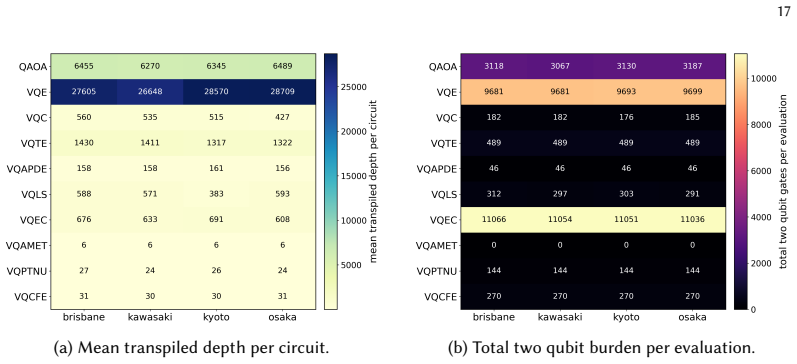
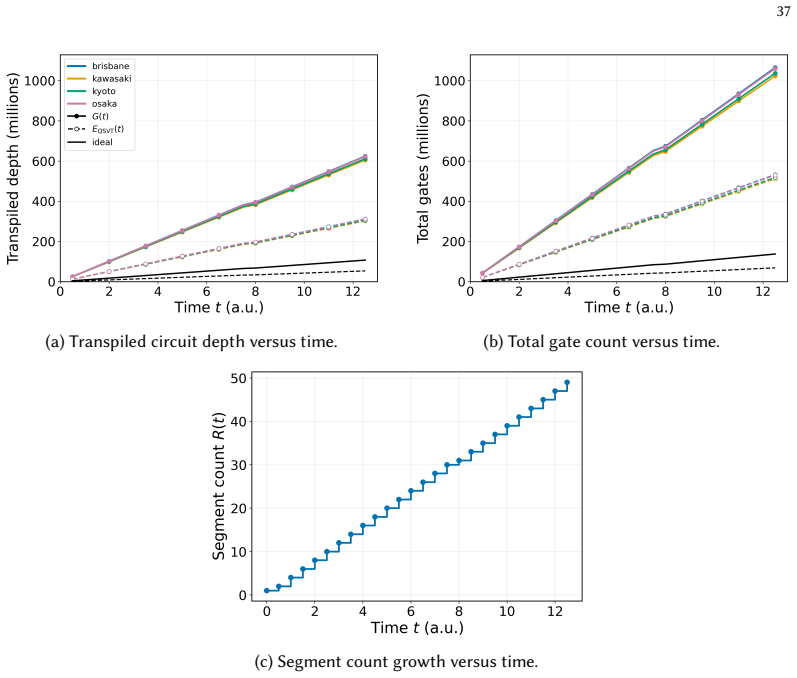
- Routed compilation cost must be read together with reliability: QSVT routed depth inflates by roughly 5.6-5.8x and total gates by 7.4-7.7x over ideal, changing the practical meaning of a backend's spectral success.
- Robust parameter regions are backend-specific in location and geometry, so noise compensation learned on one backend does not transfer unchanged to another.
Where Pith is reading between the lines
- If the same pipeline were run on live, drift-prone hardware, the rankings might reorder with calibration state; the paper's static-snapshot results give a lower bound on time-varying uncertainty, not a prediction about live-device rankings.
- The finding that sensitivity mass concentrates in a backend-specific low-dimensional subset of the 27 QSVT phases suggests a practical calibration protocol: tune only the top sensitivity coordinates per backend and fix the rest, potentially cutting optimization cost substantially.
- The LiH projection implies a gate-volume multiplier of roughly 4^6, suggesting the benchmark's real near-term value is comparative hardware characterization rather than chemistry scale-up; the same tuple pipeline could be extended to other matrix-function workloads to test whether the workload-dependence pattern is general.
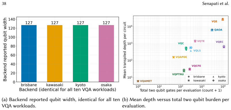
- Because VQAMET stays shallow and nearly backend-invariant while VQCFE is highly selective, workload difficulty and workload cost are separate axes; benchmark designers could stratify suites by both dimensions to avoid conflating 'hard' with 'expensive'.
Editorial analysis
A structured set of objections, weighed in public.
Referee Report
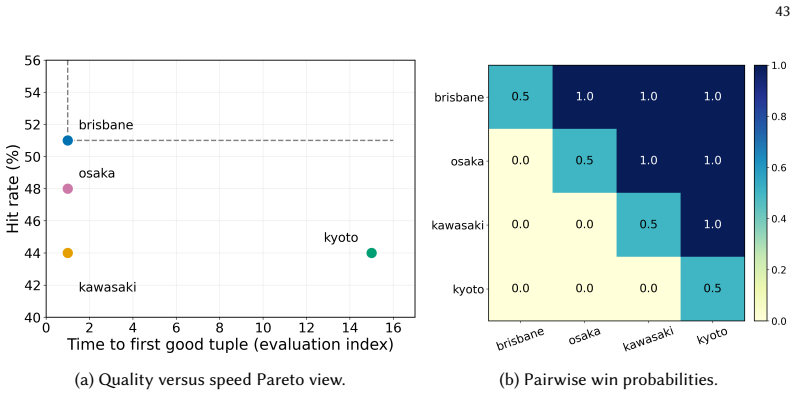
Summary. The paper presents a unified uncertainty quantification framework for application-level benchmarking of noisy quantum backends, applied to two workload classes: ten variational quantum algorithm (VQA) families and a Quantum Singular Value Transformation (QSVT) construction of the H2 Green's function. Both branches share the tuple model y_n = g_b(xi_n) + eps_n (Eq. 11) and one offline pipeline (GP surrogate, Bayesian optimization with posterior refinement, Morris/robust-density analysis, backend ranking, resource estimation). The framework is instantiated on four IBM fake backends (Brisbane, Kawasaki, Kyoto, Osaka). The headline results are workload-dependent VQA backend preferences (Brisbane best mean rank 2.38, Osaka best mean quality) and a QSVT reliability ordering Brisbane > Osaka > Kawasaki > Kyoto, based on hit rates 51/48/44/44 out of 100 evaluations and a Time-to-Good tie-break. The paper also reports sensitivity fingerprints, robust-region geometry, and transpiled resource costs, and projects the QSVT pipeline to LiH.
Significance. If the empirical claims were secured, this would be a genuinely useful contribution: it provides a common statistical language for variational and non-variational workloads; the ten VQA instances are concretely specified (Tables 5-7); the QSVT branch includes block-encoding details and a real-time segmentation error bound (App. B); the resource layer separates deep-single-circuit from many-shallow-circuits cost regimes; and the LiH projection (Eqs. 19-24) is a quantitative, falsifiable scaling prediction. The paper is also unusually explicit about scope (Sec. 5, App. J) and the workflow design (Algorithm 1, saved records, offline analysis) is reproducible in structure. However, the central empirical conclusions currently outrun the evidence: the QSVT good-tuple classifier is under-specified, the hit-rate ranking has no confidence intervals or seed variation, the VQA quality metric is relative by construction, and the sensitivity fingerprints rest on unvalidated surrogates. These are fixable within the manuscript's scope, which is why I am not recommending rejection.
major comments (5)
- [§2.4, Eq. (14), Table 8, Fig. 3] The binary good/bad classification behind every QSVT reliability number is not reproducible. A 'good tuple' is defined as one in which the guided peak loss of Eq. (14) 'reaches its lower target,' but the target value is never given; the per-peak weights w_{j,r} are never specified; and the peak distance ℓ(·,·) is only described as 'position and height aware.' Fig. 3's caption fixes only the sign symmetry min(|ω−ω_ideal|,|ω+ω_ideal|), not the tolerance in position or height. Since the hit rates in Table 8 (51/48/44/44) and the resulting ranking Brisbane > Osaka > Kawasaki > Kyoto derive entirely from this classifier, the central QSVT result cannot be independently verified. Please report the exact threshold(s) and weights, and test the stability of the ranking to variation in these choices.
- [§4.2, Table 8, App. C] The QSVT ranking rests on a single 100-evaluation adaptive trajectory per backend with no attached uncertainty. At 44/100 the binomial standard error is about 5 percentage points, so the 51/48/44/44 spread is within roughly one standard error of a common rate; the Kawasaki/Kyoto tie-break (Time-to-Good 1 vs 15) is a single-run minimum and is not a stable discriminator. Because the trajectory is adaptive, hit rate conflates backend noise with GP/acquisition/VI behavior. App. C itself notes that a beta-binomial ranking model could have been used but was not, and Fig. 17(b)'s 'pairwise win probabilities' have no stated definition or error bars. Please add seed variation, confidence intervals, and/or a model-based comparison, and re-frame the ordering as provisional.
- [§2.4, §4.1, Fig. 7, §6] quality_norm is a per-workload min-max rescaling of the best and worst observed values across the four backends, which makes all VQA aggregate rankings relative to the tested backend set and to noisy trajectory extrema. Adding or removing a backend would rescale every score, and a workload in which all four backends fail would still yield a 1.0 for the least-bad backend. The definition is stated, but the abstract's claim that the framework measures 'how reliably each backend reaches useful task level behavior' and the conclusion's 'concrete backend conclusions' overstate what this metric provides. The aggregate gaps are also small (mean ranks 2.38-2.61 over ten workloads) with no reported uncertainty. Please scope the VQA claims to relative performance within the tested set and provide bootstrap-type uncertainty over workloads and refinement settings.
- [§4.3, App. D] The Morris/Sobol/SHAP sensitivity fingerprints and robust-region densities are computed 'on surrogate models fitted to the backend evaluation records' (App. D), but no validation of the GP surrogates is reported—no cross-validated error, no comparison against direct evaluations—and 100 adaptive samples in a 27-dimensional phase space is a thin basis for global sensitivity analysis. Claims that the top-five phase block carries roughly two-thirds of the Morris mass and that the robust-region geometry is backend-specific therefore inherit unquantified surrogate error. Please report surrogate predictive accuracy and confirm the Morris ordering with a direct sampling-based estimate or a stability analysis across surrogate fits.
- [§5, App. E, §4.6, §6] The paper is appropriately explicit in §5 that all results use IBM fake-backend noise models and Aer execution rather than live QPUs, and I credit that. However, the abstract and conclusion present 'backend rankings' (e.g., 'Brisbane is the strongest backend') without re-qualifying that these are statements about static calibration snapshots. The 'transpile once, bind phases' cache of App. E is noise-faithful only because the fake backends are static; live hardware would require a refresh policy (as App. E acknowledges) and would invalidate the single-snapshot noise model. Please carry the §5 qualification into the abstract and conclusion, and state clearly that the framework has not been tested on non-stationary hardware.
minor comments (7)
- [§2.4, Table 3] Mean Eval95 is defined as reaching '95% of the per workload best value,' but the sign convention is unclear for minimization workloads where y = -f: if the best value is negative, 95% of it is a worse threshold. Please state the convention explicitly and note how negative optima are handled.
- [§2.2, §3.2] The 27-dimensional phase vector is the concatenation of the cosine-branch (13) and sine-branch (14) QSP phase vectors of the degree pair (12,13). Eq. (7) presents a single (d+1)-dimensional vector; state the concatenation explicitly so the dimension is checkable.
- [Fig. 17(b)] The 'pairwise win probabilities' have no definition in the text or caption. Specify what is being compared (evaluations? runs?) and how the probability is estimated.
- [App. J] Appendix J lists only two threats to validity (branch complementarity and breadth/tradeoff). The statistical issues affecting Table 8—single trajectory per backend, no confidence intervals, and the unspecified good-tuple threshold—are the most serious threats to the central claim and should be acknowledged there.
- [App. C / data availability] The paper states that offline analysis can be reproduced from saved evaluation records, but no data or code availability statement is provided. For a benchmarking paper, releasing the evaluation logs (or at least the aggregate tables with uncertainty) would substantially strengthen the reproducibility case.
- [§4.5, Eq. (24)] The LiH projection relies on 'the H2 fit gives roughly 2.5×10^8 routed gates at λt=5,' but this fit is not linked to any figure or table in the manuscript, so the projection is not traceable. Please state where this number comes from.
- [Table 9, §4.3] Table 9 has no paired checkpoint sets for VQLS and VQAPDE, yet §4.3 claims that VQAPDE and VQLS 'distribute their sensitivity more broadly' without noting this incompleteness. Add a cross-reference to Table 9's dashes when making sensitivity claims about those workloads.
Circularity Check
No significant circularity: all benchmark metrics are explicitly defined from recorded evaluations, and the under-specified QSVT good-tuple threshold is a reproducibility/correctness issue, not a circular reduction.
full rationale
The paper's derivation chain is a benchmarking methodology, not a predictive theory whose outputs are fed back into its definitions. The shared tuple model y_n = g_b(xi_n) + eps_n (Eq. 11) and the GP update (Eq. 16) are standard statistical machinery; the VQA and QSVT objectives are defined independently (Eqs. 1, 14). The quality_norm metric is explicitly a per-workload min-max rescaling across the four backends, so the resulting rankings are by construction relative to the tested set, but this is stated openly in Section 2.4 rather than hidden, and no claim is made that it provides an absolute external scale. The QSVT hit-rate ranking depends on the unquantified 'lower target' and per-peak weights in Eq. (14); however, the paper does not say or imply that these were fitted to produce the backend ordering, and the appendix reports raw hit rates and Time-to-Good values. An unspecified threshold is a reproducibility limitation (as the skeptic notes), not a circular step by the paper's own equations. Self-citations such as [1], [72], and [74] appear, but the central QSVT construction is also anchored in standard external references [29, 47, 48, 53] and many-body texts [27, 52], and no load-bearing uniqueness theorem is imported from the authors' prior work. The stated limitations (fake-backend noise models, qualitative noise correlations) further scope the claims rather than smuggling in conclusions. No prediction in the paper reduces to a fitted parameter or to a self-citation chain by construction, so the appropriate circularity score is 0.
Axiom & Free-Parameter Ledger
free parameters (6)
- QSVT phase vector theta (27 dimensions) =
backend-specific centers reported in Fig. 16 (figure absent)
- Per-peak weights w_{j,r} in guided peak loss Eq. (14) =
not stated
- Broadening parameter eta = 0.15 a.u. =
0.15
- Good-tuple lower target for Eq. (14) =
not stated
- alpha=0.9 level-set threshold for robust region =
0.9
- Per-workload min-max normalization range =
[0,1] with 1=best, 0=worst across four backends
axioms (5)
- domain assumption Aer fake-backend noise models are faithful proxies for the four named IBM backends.
- standard math The QSVT polynomial approximation error bound (Eq. 31) with segmentation r=ceil(tau/tau_max) is valid.
- domain assumption The H2 four-orbital Hamiltonian block encoding with three QSVT ancillas and the Hadamard-test wrapper correctly implements the retarded Green's function of Eqs. (2)-(5).
- standard math CLT justifies Gaussian per-evaluation noise in Eq. (11).
- domain assumption The LiH projection of Sect. 4.5 assumes the H2 routed-gate empirical trend is a linear proxy for LiH.
invented entities (1)
-
No new physical entities introduced.
no independent evidence
read the original abstract
We present an uncertainty quantification (UQ) framework for application level benchmarking and characterization of noisy quantum backends. The framework compares two workload classes under one statistical pipeline: noisy intermediate scale quantum (NISQ) variational quantum algorithms (VQAs) and Quantum Singular Value Transformation (QSVT) based Green's function reconstruction. For the VQA branch, we evaluate ten benchmark families spanning chemistry, optimization, simulation, compiling, linear solving, partial differential equations, metrology, error correction, tomography, and channel fidelity estimation. For the QSVT branch, we reconstruct orbital resolved Green's functions and spectral peaks from a block encoded real time propagator. The workflow combines Bayesian optimization, posterior distribution refinement, sensitivity analysis, robust parameter density estimation, backend ranking, noise correlation, and resource estimation analysis. Instead of reporting only one best parameter vector, the framework identifies robust parameter regions, residual gaps to ideal behavior, backend specific failure modes, and calibration sensitive uncertainty. The result is a common benchmark for variational and non-variational workloads that measures how reliably each backend reaches useful task level behavior.
Figures








Reference graph
Works this paper leans on
-
[1]
Vibin Abraham, Priyabrata Senapati, Himadri Pathak, and Bo Peng. 2026. Elucidating Many-Body Effects in Molecular Core Spectra through Real-Time Approaches: Efficient Classical Approximations and a Quantum Perspective.The Journal of Chemical Physics164, 10 (2026), 104113. doi:10.1063/5.0313721
-
[2]
Thomas E. Baker. 2021. Lanczos Recursion on a Quantum Computer for the Green’s Function and Ground State. Physical Review A103, 3 (2021), 032404. doi:10.1103/PhysRevA.103.032404
-
[3]
Jiang, Samuel Daulton, Benjamin Letham, Andrew Gordon Wilson, and Eytan Bakshy
Maximilian Balandat, Brian Karrer, Daniel R. Jiang, Samuel Daulton, Benjamin Letham, Andrew Gordon Wilson, and Eytan Bakshy. 2020. BoTorch: A Framework for Efficient Monte-Carlo Bayesian Optimization. InAdvances in Neural Information Processing Systems, Vol. 33. 21524–21538. arXiv:1910.06403
Pith/arXiv arXiv 2020
-
[4]
Sohaib Alam, Guillermo Alonso-Linaje, B
Ville Bergholm, Josh Izaac, Maria Schuld, Christian Gogolin, Shahnawaz Ahmed, Vishnu Ajith, M. Sohaib Alam, Guillermo Alonso-Linaje, B. AkashNarayanan, Ali Asadi, et al. 2018. PennyLane: Automatic Differentiation of Hybrid Quantum-Classical Computations. arXiv:1811.04968 [quant-ph] doi:10.48550/arXiv.1811.04968
-
[5]
Lennart Bittel and Martin Kliesch. 2021. Training Variational Quantum Algorithms Is NP-Hard.Physical Review Letters 127, 12 (2021), 120502. doi:10.1103/PhysRevLett.127.120502
-
[6]
Tizian Blatz, Joyce Kwan, Julian Léonard, and Annabelle Bohrdt. 2024. Bayesian Optimization for Robust State Preparation in Quantum Many-Body Systems.Quantum8 (2024), 1388. doi:10.22331/q-2024-06-27-1388
-
[7]
Blei, Alp Kucukelbir, and Jon D
David M. Blei, Alp Kucukelbir, and Jon D. McAuliffe. 2017. Variational Inference: A Review for Statisticians.J. Amer. Statist. Assoc.112, 518 (2017), 859–877. doi:10.1080/01621459.2017.1285773
arXiv 2017
-
[8]
Robin Blume-Kohout, Timothy Proctor, and Kevin Young. 2025. Quantum Characterization, Verification, and Validation. arXiv:2503.16383 doi:10.48550/arXiv.2503.16383
-
[9]
Robin Blume-Kohout and Kevin C. Young. 2020. A Volumetric Framework for Quantum Computer Benchmarks. Quantum4 (2020), 362. doi:10.22331/q-2020-11-15-362
-
[10]
Cerezo, Yigit Subasi, Lukasz Cincio, and Patrick J
Carlos Bravo-Prieto, Ryan LaRose, M. Cerezo, Yigit Subasi, Lukasz Cincio, and Patrick J. Coles. 2023. Variational Quantum Linear Solver.Quantum7 (2023), 1188. doi:10.22331/q-2023-11-22-1188
-
[11]
Daan Camps and Roel Van Beeumen. 2022. FABLE: Fast Approximate Quantum Circuits for Block-Encodings. InProceedings of the 2022 IEEE International Conference on Quantum Computing and Engineering (QCE). 104–113. doi:10.1109/QCE53715.2022.00029
arXiv 2022
-
[12]
Olson, Matthias Degroote, Peter D
Yudong Cao, Jonathan Romero, Jonathan P. Olson, Matthias Degroote, Peter D. Johnson, Mária Kieferová, Ian D. Kivlichan, Tim Menke, Borja Peropadre, Nicolas P. D. Sawaya, Sukin Sim, Libor Veis, and Alán Aspuru-Guzik
-
[13]
Cerezo, Andrew Arrasmith, Ryan Babbush, Simon C
M. Cerezo, Andrew Arrasmith, Ryan Babbush, Simon C. Benjamin, Suguru Endo, Keisuke Fujii, Jarrod R. McClean, Kosuke Mitarai, Xiao Yuan, Lukasz Cincio, and Patrick J. Coles. 2021. Variational Quantum Algorithms.Nature Reviews Physics3 (2021), 625–644. doi:10.1038/s42254-021-00348-9
-
[14]
Cerezo, Alexander Poremba, Lukasz Cincio, and Patrick J
M. Cerezo, Alexander Poremba, Lukasz Cincio, and Patrick J. Coles. 2020. Variational Quantum Fidelity Estimation. Quantum4 (2020), 248. doi:10.22331/q-2020-03-26-248
-
[15]
Cerezo, Akira Sone, Tyler Volkoff, Lukasz Cincio, and Patrick J
M. Cerezo, Akira Sone, Tyler Volkoff, Lukasz Cincio, and Patrick J. Coles. 2021. Cost Function Dependent Barren Plateaus in Shallow Parametrized Quantum Circuits.Nature Communications12 (2021), 1791. doi:10.1038/s41467-021- 21728-w
-
[16]
Raj Chakrabarti and Herschel Rabitz. 2007. Quantum control landscapes.International Reviews in Physical Chemistry 26, 4 (2007), 671–735. doi:10.1080/01442350701633300
-
[17]
Andrew M. Childs and Nathan Wiebe. 2012. Hamiltonian Simulation Using Linear Combinations of Unitary Operations. Quantum Information and Computation12, 11–12 (2012), 901–924. doi:10.26421/QIC12.11-12-1
-
[18]
Andrew W. Cross, Lev S. Bishop, Sarah Sheldon, Paul D. Nation, and Jay M. Gambetta. 2019. Validating Quantum Computers Using Randomized Model Circuits.Physical Review A100, 3 (2019), 032328. doi:10.1103/PhysRevA.100. 032328 23
-
[19]
Diksha Dhawan, Dominika Zgid, and Mario Motta. 2024. Quantum Algorithm for Imaginary-Time Green’s Functions. Journal of Chemical Theory and Computation20, 11 (2024), 4629–4638. doi:10.1021/acs.jctc.4c00241
-
[20]
Daoyi Dong and Ian R Petersen. 2010. Quantum control theory and applications: a survey.IET Control Theory & Applications4, 12 (2010), 2651–2671. doi:10.1049/iet-cta.2009.0508
arXiv 2010
-
[21]
Yulong Dong, Lin Lin, and Yu Tong. 2022. Ground-State Preparation and Energy Estimation on Early Fault-Tolerant Quantum Computers via Quantum Eigenvalue Transformation of Unitary Matrices.PRX Quantum3, 4 (2022), 040305. doi:10.1103/PRXQuantum.3.040305
-
[22]
J. Eisert, D. Hangleiter, N. Walk, I. Roth, D. Markham, R. Parekh, U. Chabaud, and E. Kashefi. 2020. Quantum Certification and Benchmarking.Nature Reviews Physics2, 7 (2020), 382–390. doi:10.1038/s42254-020-0186-4
-
[23]
Suguru Endo, Ikko Kurata, and Yuya O. Nakagawa. 2020. Calculation of the Green’s Function on Near-Term Quantum Computers.Physical Review Research2, 3 (2020), 033281. doi:10.1103/PhysRevResearch.2.033281
-
[24]
Wallman, Lukas Postler, Michael Meth, Roman Stricker, Esteban A
Alexander Erhard, Joel J. Wallman, Lukas Postler, Michael Meth, Roman Stricker, Esteban A. Martinez, Philipp Schindler, Thomas Monz, Joseph Emerson, and Rainer Blatt. 2019. Characterizing Large-Scale Quantum Computers via Cycle Benchmarking.Nature Communications10 (2019), 5347. doi:10.1038/s41467-019-13068-7
-
[25]
Turner, and Matthias Poloczek
David Eriksson, Michael Pearce, Jacob Gardner, Ryan D. Turner, and Matthias Poloczek. 2019. Scalable Global Optimization via Local Bayesian Optimization. InAdvances in Neural Information Processing Systems
2019
-
[26]
Edward Farhi, Jeffrey Goldstone, and Sam Gutmann. 2014. A Quantum Approximate Optimization Algorithm. arXiv:1411.4028. doi:10.48550/arXiv.1411.4028
-
[27]
Fetter and John D
Alexander L. Fetter and John D. Walecka. 2003.Quantum Theory of Many-Particle Systems. Dover
2003
-
[28]
Stepan Fomichev, Pablo A. M. Casares, Jay Soni, Utkarsh Azad, Alexandr Kunitsa, Arne-Christian Voigt, Jonathan E. Mueller, and Juan Miguel Arrazola. 2025. Fast Simulations of X-Ray Absorption Spectroscopy for Battery Materials on a Quantum Computer. doi:10.48550/arXiv.2506.15784
-
[29]
András Gilyén, Yuan Su, Guang Hao Low, and Nathan Wiebe. 2019. Quantum Singular Value Transformation and Beyond: Exponential Improvements for Quantum Matrix Arithmetics. InProceedings of the 51st Annual ACM SIGACT Symposium on Theory of Computing. 193–204. doi:10.1145/3313276.3316366
arXiv 2019
-
[30]
Niladri Gomes, David B. Williams-Young, and Wibe A. de Jong. 2023. Computing the Many-Body Green’s Function with Adaptive Variational Quantum Dynamics.Journal of Chemical Theory and Computation19, 11 (2023), 3313–3323. doi:10.1021/acs.jctc.3c00150
-
[31]
Gabriel Greene-Diniz, David Zsolt Manrique, Kentaro Yamamoto, Evgeny Plekhanov, Nathan Fitzpatrick, Michal Krompiec, Rei Sakuma, and David Muñoz Ramo. 2024. Quantum Computed Green’s Functions Using a Cumulant Expansion of the Lanczos Method.Quantum8 (2024), 1383. doi:10.22331/q-2024-06-20-1383
-
[32]
Nguyen, Noah Goss, Brian Marinelli, Ravi K
Akel Hashim, Long B. Nguyen, Noah Goss, Brian Marinelli, Ravi K. Naik, Trevor Chistolini, Jordan Hines, J. P. Marceaux, Yosep Kim, Pranav Gokhale, Teague Tomesh, Senrui Chen, Liang Jiang, Samuele Ferracin, Kenneth Rudinger, Timothy Proctor, Kevin C. Young, Irfan Siddiqi, and Robin Blume-Kohout. 2025. Practical Introduction to Benchmarking and Characteriza...
-
[33]
Zoë Holmes, Kunal Sharma, M. Cerezo, and Patrick J. Coles. 2022. Connecting Ansatz Expressibility to Gradient Magnitudes and Barren Plateaus.PRX Quantum3, 1 (2022), 010313. doi:10.1103/PRXQuantum.3.010313
-
[34]
Wood, Jake Lishman, Julien Gacon, Simon Martiel, Paul D
Ali Javadi-Abhari, Matthew Treinish, Kevin Krsulich, Christopher J. Wood, Jake Lishman, Julien Gacon, Simon Martiel, Paul D. Nation, Lev S. Bishop, Andrew W. Cross, Blake R. Johnson, and Jay M. Gambetta. 2024. Quantum Computing with Qiskit. arXiv:2405.08810 doi:10.48550/arXiv.2405.08810
-
[35]
Jones, Matthias Schonlau, and William J
Donald R. Jones, Matthias Schonlau, and William J. Welch. 1998. Efficient Global Optimization of Expensive Black-Box Functions.Journal of Global Optimization13, 4 (1998), 455–492. doi:10.1023/A:1008306431147
-
[36]
Nakagawa, Kazunori Maruyama, Hirotaka Oshima, and Shintaro Sato
Shota Kanasugi, Shoichiro Tsutsui, Yuya O. Nakagawa, Kazunori Maruyama, Hirotaka Oshima, and Shintaro Sato
-
[37]
Abhinav Kandala, Antonio Mezzacapo, Kristan Temme, Maika Takita, Markus Brink, Jerry M. Chow, and Jay M. Gambetta. 2017. Hardware-Efficient Variational Quantum Eigensolver for Small Molecules and Quantum Magnets. Nature549, 7671 (2017), 242–246. doi:10.1038/nature23879
-
[38]
Trevor Keen, Bo Peng, Karol Kowalski, Pavel Lougovski, and Steven Johnston. 2022. Hybrid Quantum-Classical Approach for Coupled-Cluster Green’s Function Theory.Quantum6 (2022), 675. doi:10.22331/q-2022-03-30-675
-
[39]
Sumeet Khatri, Ryan LaRose, Alexander Poremba, Lukasz Cincio, Andrew T. Sornborger, and Patrick J. Coles. 2019. Quantum-Assisted Quantum Compiling.Quantum3 (2019), 140. doi:10.22331/q-2019-05-13-140
-
[40]
Knill, D
E. Knill, D. Leibfried, R. Reichle, J. Britton, R. B. Blakestad, J. D. Jost, C. Langer, R. Ozeri, S. Seidelin, and D. J. Wineland
-
[41]
Taichi Kosugi and Yu-ichiro Matsushita. 2020. Construction of Green’s Functions on a Quantum Computer: Quasipar- ticle Spectra of Molecules.Physical Review A101, 1 (2020), 012330. doi:10.1103/PhysRevA.101.012330 24 Senapati et al
-
[42]
Bauman, Guang Hao Low, Martin Roetteler, John J
Karol Kowalski, Nicholas P. Bauman, Guang Hao Low, Martin Roetteler, John J. Rehr, and Fernando D. Vila. 2024. Capturing Many-Body Correlation Effects with Quantum and Classical Computing.Physical Review A110, 6 (2024), L060401. doi:10.1103/PhysRevA.110.L060401
-
[43]
Alexandr Kunitsa, Diksha Dhawan, Stepan Fomichev, Juan Miguel Arrazola, Minghao Zhang, and Torin F. Stetina
-
[44]
Coles, Lukasz Cincio, Jarrod R
Martín Larocca, Supanut Thanasilp, Samson Wang, Kunal Sharma, Jacob Biamonte, Patrick J. Coles, Lukasz Cincio, Jarrod R. McClean, Zoë Holmes, and M. Cerezo. 2025. Barren Plateaus in Variational Quantum Computing.Nature Reviews Physics(2025). doi:10.1038/s42254-025-00813-9
-
[45]
Marjuka F Lazin, Christian R Shelton, Simon N Sandhofer, and Bryan M Wong. 2023. High-dimensional multi-fidelity Bayesian optimization for quantum control.Mach. Learn.: Sci. Technol.4, 4 (2023), 045014. doi:10.1088/2632-2153/ad0100
-
[46]
Francesco Libbi, Jacopo Rizzo, Francesco Tacchino, Nicola Marzari, and Ivano Tavernelli. 2022. Effective Calculation of the Green’s Function in the Time Domain on Near-Term Quantum Processors.Physical Review Research4, 4 (2022), 043038. doi:10.1103/PhysRevResearch.4.043038
-
[47]
Guang Hao Low and Isaac L. Chuang. 2017. Optimal Hamiltonian Simulation by Quantum Signal Processing.Physical Review Letters118, 1 (2017), 010501. doi:10.1103/PhysRevLett.118.010501
-
[48]
Guang Hao Low and Isaac L. Chuang. 2019. Hamiltonian Simulation by Qubitization.Quantum3 (2019), 163. doi:10.22331/q-2019-07-12-163
-
[49]
Baldwin, Karl Mayer, and Timothy Proctor
Thomas Lubinski, Sonika Johri, Paul Varosy, Jeremiah Coleman, Luning Zhao, Jason Necaise, Charles H. Baldwin, Karl Mayer, and Timothy Proctor. 2023. Application-Oriented Performance Benchmarks for Quantum Computing.IEEE Transactions on Quantum Engineering4 (2023), 1–35. doi:10.1109/TQE.2023.3253761
arXiv 2023
-
[50]
Scott M Lundberg and Su-In Lee. 2017. A unified approach to interpreting model predictions.Advances in neural information processing systems30 (2017)
2017
-
[51]
Easwar Magesan, Jay M. Gambetta, and Joseph Emerson. 2011. Scalable and Robust Randomized Benchmarking of Quantum Processes.Physical Review Letters106, 18 (2011), 180504. doi:10.1103/PhysRevLett.106.180504
-
[52]
Gerald D. Mahan. 2000.Many-Particle Physics(3 ed.). Springer
2000
-
[53]
John M. Martyn, Zane M. Rossi, Andrew K. Tan, and Isaac L. Chuang. 2021. Grand Unification of Quantum Algorithms. PRX Quantum2, 4 (2021), 040203. doi:10.1103/PRXQuantum.2.040203
-
[54]
McClean, Jonathan Romero, Ryan Babbush, and Alán Aspuru-Guzik
Jarrod R. McClean, Jonathan Romero, Ryan Babbush, and Alán Aspuru-Guzik. 2016. The Theory of Variational Hybrid Quantum-Classical Algorithms.New Journal of Physics18, 2 (2016), 023023. doi:10.1088/1367-2630/18/2/023023
-
[55]
Johannes Jakob Meyer, Johannes Borregaard, and Jens Eisert. 2021. A Variational Toolbox for Quantum Multi-Parameter Estimation.npj Quantum Information7 (2021), 89. doi:10.1038/s41534-021-00425-y
-
[56]
K. Mitarai, M. Negoro, M. Kitagawa, and K. Fujii. 2018. Quantum Circuit Learning.Physical Review A98, 3 (2018), 032309. doi:10.1103/PhysRevA.98.032309
-
[57]
Mooney, Gregory A
Gary J. Mooney, Gregory A. L. White, Charles D. Hill, and Lloyd C. L. Hollenberg. 2021. Whole-Device Entanglement in a 65-Qubit Superconducting Quantum Computer.Advanced Quantum Technologies4, 7 (2021), 2100061. doi:10.1002/ qute.202100061
2021
-
[58]
Max D. Morris. 1991. Factorial Sampling Plans for Preliminary Computational Experiments.Technometrics33, 2 (1991), 161–174. doi:10.1080/00401706.1991.10484804
arXiv 1991
-
[59]
Rick Mukherjee, Frédéric Sauvage, Harry Xie, Robert Löw, and Florian Mintert. 2020. Preparation of ordered states in ultra-cold gases using Bayesian optimization.New Journal of Physics22, 7 (2020), 075001. doi:10.1088/1367-2630/ab8677
-
[60]
Erik Nielsen, John King Gamble, Kenneth Rudinger, Travis Scholten, Kevin Young, and Robin Blume-Kohout. 2021. Gate Set Tomography.Quantum5 (2021), 557. doi:10.22331/q-2021-10-05-557
-
[61]
Love, Alán Aspuru-Guzik, and Jeremy L
Alberto Peruzzo, Jarrod McClean, Peter Shadbolt, Man-Hong Yung, Xiao-Qi Zhou, Peter J. Love, Alán Aspuru-Guzik, and Jeremy L. O’Brien. 2014. A Variational Eigenvalue Solver on a Photonic Quantum Processor.Nature Communications 5 (2014), 4213. doi:10.1038/ncomms5213
-
[62]
Timothy Proctor, Stefan Seritan, Kenneth Rudinger, Erik Nielsen, Robin Blume-Kohout, and Kevin Young. 2022. Scalable Randomized Benchmarking of Quantum Computers Using Mirror Circuits.Physical Review Letters129, 15 (2022), 150502. doi:10.1103/PhysRevLett.129.150502
-
[63]
Carl Edward Rasmussen and Christopher K. I. Williams. 2006.Gaussian Processes for Machine Learning. MIT Press
2006
-
[64]
Ollitrault, Nicola Marzari, and Ivano Tavernelli
Jacopo Rizzo, Francesco Libbi, Francesco Tacchino, Pauline J. Ollitrault, Nicola Marzari, and Ivano Tavernelli. 2022. One-Particle Green’s Functions from the Quantum Equation of Motion Algorithm.Physical Review Research4, 4 (2022), 043011. doi:10.1103/PhysRevResearch.4.043011
-
[65]
Andrea Saltelli, Paola Annoni, Ivano Azzini, Francesca Campolongo, Marco Ratto, and Stefano Tarantola. 2010. Variance Based Sensitivity Analysis of Model Output. Design and Estimator for the Total Sensitivity Index.Computer Physics Communications181, 2 (2010), 259–270. doi:10.1016/j.cpc.2009.09.018 25
-
[66]
Yuki Sato, Ruho Kondo, Satoshi Koide, Hideki Takamatsu, and Nobuyuki Imoto. 2021. Variational Quantum Algorithm Based on the Minimum Potential Energy for Solving the Poisson Equation.Physical Review A104, 5 (2021), 052409. doi:10.1103/PhysRevA.104.052409
-
[67]
Frédéric Sauvage and Florian Mintert. 2020. Optimal Quantum Control with Poor Statistics.PRX Quantum1, 2 (2020), 020322. doi:10.1103/PRXQuantum.1.020322
-
[68]
Maria Schuld, Ryan Sweke, and Johannes Jakob Meyer. 2021. Effect of Data Encoding on the Expressive Power of Variational Quantum-Machine-Learning Models.Physical Review A103, 3 (2021), 032430. doi:10.1103/PhysRevA.103. 032430
-
[69]
Athawale, David Pugmire, and Qiang Guan
Priyabrata Senapati, Tushar M. Athawale, David Pugmire, and Qiang Guan. 2023. Advancing Comprehension of Quantum Application Outputs: A Visualization Technique. InQCCC 2023 - Proceedings of the 2023 International Workshop on Quantum Classical Cooperative Computing. 25–28. doi:10.1145/3588983.3596689
arXiv 2023
-
[70]
Athawale, Ang Li, Weiwen Jiang, Zhepeng Wang, Qiang Guan, and Cheng Chang Lu
Priyabrata Senapati, Samuel Yen-Chi Chen, Bo Fang, Tushar M. Athawale, Ang Li, Weiwen Jiang, Zhepeng Wang, Qiang Guan, and Cheng Chang Lu. 2024. PQML: Enabling the Predictive Reproducibility on NISQ Machines for Quantum ML Applications. InProceedings of the 2024 IEEE International Conference on Quantum Computing and Engineering (QCE). 1413–1424. doi:10.11...
arXiv 2024
-
[71]
Priyabrata Senapati, Qiang Guan, David Pugmire, Cheng Chang Lu, and Tushar M. Athawale. 2025. Visualization of Noisy and Less Noisy Computational Basis States in Quantum Computing. InProceedings of the 2025 IEEE International Conference on Quantum Software (QSW). 12–21. doi:10.1109/QSW67625.2025.00011
arXiv 2025
-
[72]
Priyabrata Senapati, Waylon Luo, Bo Peng, and Qiang Guan. 2026. Uncertainty Quantification Driven Benchmarking and Characterization of Noisy Quantum Backends: A VQE Case Study. InProceedings of the Great Lakes Symposium on VLSI 2026 (GLSVLSI ’26). Association for Computing Machinery, New York, NY, USA, 830–835. doi:10.1145/3787109. 3816378
-
[73]
Humble, Bo Fang, Shuai Xu, and Qiang Guan
Priyabrata Senapati, Zhepeng Wang, Weiwen Jiang, Travis S. Humble, Bo Fang, Shuai Xu, and Qiang Guan. 2023. Towards Redefining the Reproducibility in Quantum Computing: A Data Analysis Approach on NISQ Devices. InProceedings of the 2023 IEEE International Conference on Quantum Computing and Engineering (QCE). 468–474. doi:10.1109/QCE57702.2023.00060
arXiv 2023
-
[74]
Priyabrata Senapati, Shengye Zhu, Bo Peng, Bo Fang, and Qiang Guan. 2025. UQ-VarQA: Benchmarking and Charac- terizing NISQ Computers through Uncertainty Quantification of Variational Quantum Algorithms. InProceedings of the 2025 IEEE 43rd International Conference on Computer Design (ICCD). 356–363. doi:10.1109/ICCD65941.2025.00058
arXiv 2025
-
[75]
Bobak Shahriari, Kevin Swersky, Ziyu Wang, Ryan P. Adams, and Nando de Freitas. 2016. Taking the Human Out of the Loop: A Review of Bayesian Optimization.Proc. IEEE104, 1 (2016), 148–175. doi:10.1109/JPROC.2015.2494218
arXiv 2016
-
[76]
B. W. Silverman. 1986.Density Estimation for Statistics and Data Analysis. Chapman & Hall
1986
-
[77]
Jasper Snoek, Hugo Larochelle, and Ryan P. Adams. 2012. Practical Bayesian Optimization of Machine Learning Algorithms. InAdvances in Neural Information Processing Systems
2012
-
[78]
Sullivan
Timothy J. Sullivan. 2015.Introduction to Uncertainty Quantification. Springer
2015
-
[79]
Jules Tilly, Hongxiang Chen, Shuxiang Cao, Dario Picozzi, Kanav Setia, Ying Li, Edward Grant, Leonard Wossnig, Ivan Rungger, George H. Booth, and Jonathan Tennyson. 2022. The Variational Quantum Eigensolver: A Review of Methods and Best Practices.Physics Reports986 (2022), 1–128. doi:10.1016/j.physrep.2022.08.003
-
[80]
Smith, Joshua Viszlai, Xin Chuan Wu, Nikos Hardavellas, Margaret R
Teague Tomesh, Pranav Gokhale, Victory Omole, Gokul Subramanian Ravi, Kaitlin N. Smith, Joshua Viszlai, Xin Chuan Wu, Nikos Hardavellas, Margaret R. Martonosi, and Frederic T. Chong. 2022. SupermarQ: A Scalable Quantum Benchmark Suite. InProceedings of the 2022 IEEE International Symposium on High-Performance Computer Architecture (HPCA). 587–603. doi:10....
arXiv 2022
discussion (0)
Sign in with ORCID, Apple, or X to comment. Anyone can read and Pith papers without signing in.