REVIEW 3 major objections 5 minor 27 references
Cost-blind credit can forfeit nearly all attainable quality in LLM discovery search; CostAda restores it with budget-conditioned, cost-calibrated utility.
Reviewed by Pith at T0; open to challenge. T0 means a machine referee read the full paper against a public rubric. the ladder, T0–T4 →
T0 review · deepseek-v4-flash
2026-08-01 10:42 UTC pith:34UYILYE
load-bearing objection Clean separation proof and a coherent cost-aware controller, but the empirical 12/16 claim currently rests on unstated hyperparameter values and three-seed runs; worth reviewing once the numbers and tuning protocol are on the table. the 3 major comments →
Budget-Aware LLM Discovery via Cost-Calibrated Frontier Utility
The pith
A machine-rendered reading of the paper's core claim, the machinery that carries it, and where it could break.
Core claim
The central claim is that search-side cost must be part of the credit signal, not an accounting side note. Under a fixed budget, the relevant objective is best-so-far quality before the ledger runs out. The paper proves, as Proposition 1, that for any cost ratio κ > 1 and K ≥ 2 frontiers, there exists an equal-gain instance—one cheap frontier earning the same score increment as K − 1 expensive ones—in which every cost-blind controller attains at most (1/K + 1/κ)(1 + o(1)) of optimal budgeted value, while a gain-per-cost ranking attains (1 − o(1)). This formalizes the intuition that score-only credit cannot tell cheap productivity from expensive waste when every step yields the same score ris
What carries the argument
The load-bearing object is the cost-calibrated frontier utility u = (λ g + (1 − λ) δ) / (1 + λ_c log(1 + c_norm)), where δ is normalized local gain against a frontier's own archive, g is normalized global gain over the best-so-far solution, λ = 1 − ρ rises as the remaining-budget ratio ρ falls, and c_norm is normalized realized cost. It does three things at once: it discounts progress by realized cost, it shifts credit from local development to global improvement as the budget drains, and it feeds three coupled decisions—local exploration intensity, frontier allocation by global gain per realized cost, and budgeted tactic intervention gated on affordability and evidence. A smoothed version o
Load-bearing premise
The empirical half-budget advantage rests on the controller constants being fixed without tuning on the eight benchmarks and fully specified; the paper states their roles but gives no numeric values or tuning protocol, so the 12-of-16 result could be an artifact of selection if those constants were chosen on the same data.
What would settle it
Construct the Proposition 1 instance with K=4 frontiers, cost ratio κ=10, and a long horizon; run any cost-blind controller against gain-per-cost allocation, and compare expected best-so-far quality to OPT. If the cost-blind controller does not approach the (1/4 + 1/10) fraction, the theorem's construction fails. For the empirical claim, re-run CostAda on the eight benchmarks with the constants re-tuned on a separate benchmark family and check whether the 12-of-16 half-budget margin survives.
If this is right
- Under heterogeneous action costs, progress-only credit becomes asymptotically insufficient as frontiers multiply; smoothing or optimism adjustments do not rescue it (Proposition 1).
- Budget-matched final quality does not require a larger ledger; redirecting credit by realized cost and remaining budget changes where the same dollars go.
- A controller that conditions on remaining budget behaves differently early and late: the same expensive step can be worth buying near the start and not near the horizon.
- Cost and remaining budget can act as control inputs for exploration, allocation, and intervention rather than only as a stopping rule, which is the design principle CostAda instantiates.
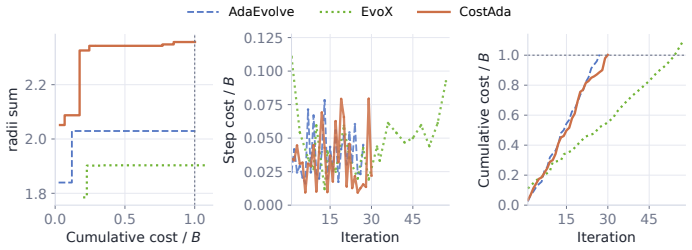
- At most half the budget buys the strongest baseline's full-budget quality in twelve of sixteen benchmark–backbone pairs, and the mean final quality is strongest on all eight benchmarks under both backbones.
Where Pith is reading between the lines
- If the Proposition 1 separation generalizes beyond equal-gain constructions, then any discovery system that counts iterations or samples as comparable units may be systematically misallocating budget; cost-calibrated credit is a general remedy worth testing in other evaluator-driven search settings.
- The theory suggests a quantitative prediction: the advantage of cost-calibrated allocation over cost-blind allocation should grow with the cost spread among actions and with the number of frontiers; running the same protocol at several price ratios would test whether the 12-of-16 result is driven by that spread.
- Reporting normalized AUC over the budget path, as this paper does, could become a standard way to compare discovery controllers, because it rewards reaching quality early rather than only at the endpoint.
- One direct extension is to make the utility's cost penalty adaptive to the empirical cost distribution rather than fixed floors, which could help when action costs are heavy-tailed.
Editorial analysis
A structured set of objections, weighed in public.
Referee Report
Summary. The paper studies LLM-guided discovery under a fixed search-side token cost budget. It argues that existing controllers assign credit from score progress alone, ignoring the realized cost of actions, and proposes CostAda, a controller built on a cost-calibrated frontier utility (Eq. 1) that combines local and global score gains with a remaining-budget-dependent weight and divides by a log-scaled realized cost. CostAda uses this utility to control local exploration intensity, frontier allocation, and budgeted tactic intervention. The paper contributes a formal separation result (Proposition 1): on an equal-gain K-frontier instance with one cheap frontier and K-1 expensive frontiers, every cost-blind controller attains at most (1/K + 1/κ)(1+o(1)) of the optimal budgeted objective, while a gain-per-cost ranking attains (1-o(1)) OPT. Empirically, the paper claims that CostAda reaches the strongest baseline's full-budget quality with at most half the budget on twelve of sixteen benchmark–backbone pairs and records the strongest mean final quality on all eight benchmarks under GLM-5 and GPT-5.4.
Significance. Proposition 1 is a clean, correct worst-case argument and is the paper's strongest contribution: it identifies a real failure mode of progress-only credit under heterogeneous costs and gives a concrete condition under which the budgeted objective is lost. The CostAda design is coherent, and the component ablations in Appendix G support the role of each mechanism in-sample. If the empirical claims were backed by reproducible controller settings and calibrated statistical evidence, the paper would be a genuinely useful contribution to budget-aware LLM search. As it stands, the empirical half-budget headline is not sufficiently supported by the manuscript: the controller constants are not reported, and the claims rest on three runs per cell without significance testing or confidence intervals.
major comments (3)
- [§B.5, Table 3; Reproducibility Statement] The controller constants (α, γ, λmin, cucb, εg, ν0, Imin/Imax, εc, εH, ĉguide) are listed only by role; no numeric values or tuning protocol are given. This matters because the empirical headlines—12/16 half-budget matches and strongest mean on all eight benchmarks—are produced by CostAda with these constants, and Proposition 1 does not constrain them. The statement in §B.5 that constants are 'fixed within each benchmark family and are not retuned per benchmark' is ambiguous: if 'family' means the eight-benchmark suite, the statement still does not say how the values were chosen before seeing the benchmarks; if it means per-benchmark family, the claim is weaker. The Reproducibility Statement asserts that 'controller settings' are provided, which the manuscript does not do. Please supply the exact values (or a precise pointer to them in the code archive), a description of how they were ch
- [§5.1, Table 1; Appendix E] Only three runs are used per benchmark–method cell, and no significance tests, bootstrap intervals, or effect-size measures are reported. Many of the reported wins are small relative to the dispersion. For example, under GLM-5, Heilbronn Triangle is 0.0314±0.0003 vs. AdaEvolve 0.0303±0.0011, and MinMaxDist (n=16,d=2) is 13.11±0.29 vs. EvoX 14.17±1.92; in both cases the margins are within one standard deviation of the baselines. The categorical statements 'strongest mean final quality on all eight benchmarks' and 'twelve of sixteen' treat sample means as population conclusions. Please report paired permutation tests or bootstrap confidence intervals across the three seeds (and, ideally, additional seeds) for the per-benchmark comparisons, and state which of the twelve pairs remain significant at a reasonable threshold.
- [§5.3, Tables 6–7; Appendix F] The headline 'at most half the budget' is computed by reading full-budget CostAda trajectories at a 0.5B cutoff and comparing their means to the strongest baseline's full-budget mean. That is a legitimate observational claim, but it is not the same as running CostAda with a half-budget planning horizon. The independent small-budget reruns in Appendix F are reassuring, but the main text's 12/16 number is still the cutoff-based number, and the appendix reruns are also reported without uncertainty. Please make clear which of the two quantities is the primary claim and report uncertainty for both. If the primary claim is the cutoff-based one, a sentence explaining why the independent rerun result is not used as the headline would help.
minor comments (5)
- [§4.2, Eq. (1)] The terminology 'cost-calibrated frontier utility' is used even though the utility is a design choice rather than a fitted or calibrated quantity. Consider calling it 'cost-adjusted' or 'cost-normalized' to avoid implying that calibration was performed.
- [§5.3] The sentence 'CostAda leads or ties 30 of the 32 benchmark-objective cells under GLM-5' should be cross-checked against Appendix E: the appendix reports normalized-score cells in Appendix H and benchmark-objective cells in Tables 6–7. The main text should state which table supports the count.
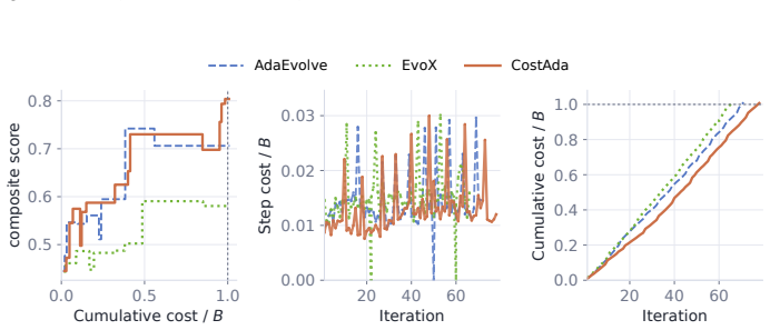
- [Figure 4] The left panel axis label 'composite score' is not defined in the caption; in Section 5.4 the text refers to 'best-so-far benchmark objective'. Please align the caption with the text.
- [§B.5] Table 3 lists ĉguide as a constant, but the text says the low-yield criterion uses 'an estimated guide call' cost. If ĉguide is estimated from the same benchmark family, describe how the estimate is formed; otherwise the term 'estimate' is misleading.
- [Appendix F] The independent small-budget reruns are described as being configured with nominal budget B=0.5, but the baseline trajectories for comparison are still the full-budget runs read at cutoffs. A direct comparison with baselines also run at B=0.5 would be cleaner.
Circularity Check
No significant circularity: Proposition 1 is self-contained, Eq. (1) is a design choice, and the empirical claims are measured rather than derived from fitted constants.
full rationale
The paper's derivation chain is self-contained. Proposition 1 is an adversarial construction with equal per-step gains and one cheap frontier; the upper bound for cost-blind controllers is proven from the ledger constraint and the identity Σ_j V_j(N_max)=N_max, while the achievability direction is an explicit policy that selects every frontier once to identify the cheap frontier and then selects it. Neither direction assumes its conclusion. The cost-calibrated frontier utility in Eq. (1) is presented as a design choice, not as a quantity fitted to the benchmarks, and the subsequent controls are defined in terms of it rather than derived from the experimental outcomes. The empirical claim that CostAda reaches the strongest baseline's full-budget quality at half the budget is a measured comparison on shared evaluators, prices, and budgets, not a prediction reconstructed from the controller constants. The paper does not invoke a load-bearing self-citation: its theoretical result is proved in the appendix, and the baseline comparisons cite prior work by other groups. The absence of numeric values or a tuning protocol for the Table 3 constants is a reproducibility concern and a possible source of selection bias, but it is not an instance where a fitted input is renamed as a prediction within the derivation; the constants are not shown to be fitted to the reported benchmarks. No circular step meeting the quoted-evidence standard was found.
Axiom & Free-Parameter Ledger
free parameters (10)
- α (utility smoothing rate)
- γ (allocation smoothing rate)
- λmin (cost-penalty floor)
- cucb (optimism scale)
- ϵg (meaningful-progress threshold)
- ϵinc (incumbent-level threshold) =
10ϵg
- ν0 (base patience scale)
- Imin, Imax (local intensity bounds)
- ĉguide (guide-cost estimate)
- ϵc, ϵH (numerical stabilizers)
axioms (6)
- domain assumption Deterministic scalar evaluator F: P → R exists and is the only quality feedback
- domain assumption Search-side LLM cost is additive and observed only after the call returns
- domain assumption Frontier representation with local archives and a global best is a faithful model of AdaEvolve/EvoX-style discovery
- standard math UCB-style optimism bounds apply to smoothed allocation rewards
- domain assumption Runs may overshoot the nominal budget by the crossing iteration's cost
- domain assumption The eight benchmarks are representative of LLM discovery and the fixed constants generalize
read the original abstract
Large language models increasingly support scientific and algorithmic discovery through inference-time search over evaluated candidates. Existing adaptive discovery controllers assign credit based only on score progress, even though prompt length, retries, and guidance calls cause search actions to incur different token costs. We prove that cost-blind credit can forfeit all but a vanishing fraction of attainable quality as frontiers multiply and costs diverge. Under a fixed search-side token budget, the controller must decide which frontier is improving and whether its gain justifies the realized cost before the budget is exhausted. We introduce \textbf{CostAda}, a cost-calibrated adaptive controller built around \emph{cost-calibrated frontier utility}. The utility values frontier progress relative to realized action cost and conditions that credit on the remaining budget. CostAda uses this signal to control local exploration intensity, frontier allocation, and budgeted tactic intervention. Cost and remaining budget therefore shape the search rather than serving only as accounting variables or a stopping rule. CostAda reaches the strongest baseline's full-budget quality with at most half the budget on twelve of sixteen benchmark--backbone pairs while achieving the strongest mean final quality on all eight benchmarks under GLM-5 and GPT-5.4.
Figures






Reference graph
Works this paper leans on
-
[1]
The art of scaling test-time compute for large language models.arXiv preprint arXiv:2512.02008,
Aradhye Agarwal, Ayan Sengupta, and Tanmoy Chakraborty. The art of scaling test-time compute for large language models.arXiv preprint arXiv:2512.02008,
-
[3]
Mohammad Ali Alomrani, Yingxue Zhang, Derek Li, Qianyi Sun, Soumyasundar Pal, Zhanguang Zhang, Yaochen Hu, Rohan Deepak Ajwani, Antonios Valkanas, Raika Karimi, Peng Cheng, Yunzhou Wang, Pengyi Liao, Hanrui Huang, Bin Wang, Jianye Hao, and Mark Coates. Reasoning on a budget: A survey of adaptive and controllable test-time compute in llms.arXiv preprint ar...
-
[4]
Henrique Assumpção, Diego Ferreira, Leandro Campos, and Fabricio Murai. CodeEvolve: An open source evolutionary coding agent for algorithm discovery and optimization.arXiv preprint arXiv:2510.14150,
-
[6]
Ties at the reported precision are jointly bolded
Best entries within each benchmark and cutoff are bolded. Ties at the reported precision are jointly bolded. Benchmark MethodB=0.25B=0.5B=0.75B=1 Circle Packing AdaEvolve 0.6917±0.0844 0.9370±0.0593 0.9722±0.0293 0.9722±0.0293 EvoX 0.8279±0.0304 0.9536±0.0481 0.9760±0.0285 0.9760±0.0285 CostAda0.9691±0.0222 0.9873±0.0127 0.9963±0.0036 0.9983±0.0021 Circle...
arXiv 2042
-
[7]
Ties at the reported precision are jointly bolded
Best entries within each benchmark and cutoff are bolded. Ties at the reported precision are jointly bolded. Benchmark Method0.25B0.5B0.75B1B Circle Packing AdaEvolve 0.9727±0.0297 0.9801±0.0194 0.9816±0.0203 0.9941±0.0011 EvoX 0.9573±0.0125 0.9655±0.0231 0.9798±0.0181 0.9811±0.0193 CostAda0.9921±0.0053 0.9947±0.0012 0.9950±0.0017 0.9961±0.0017 Circle Pac...
-
[9]
Automated design of agentic systems
Shengran Hu, Cong Lu, and Jeff Clune. Automated design of agentic systems. InInternational Conference on Learning Representations, volume 2025, pp. 21344–21377,
2025
-
[10]
Jiachen Jiang, Tianyu Ding, and Zhihui Zhu. DeltaEvolve: Accelerating scientific discovery through momentum-driven evolution.arXiv preprint arXiv:2602.02919,
-
[11]
Robert Tjarko Lange, Yuki Imajuku, and Edoardo Cetin. ShinkaEvolve: Towards open-ended and sample-efficient program evolution.arXiv preprint arXiv:2509.19349,
-
[12]
SelfBudgeter: Adaptive token allocation for efficient LLM reasoning.arXiv preprint arXiv:2505.11274,
Zheng Li, Qingxiu Dong, Jingyuan Ma, Di Zhang, Kai Jia, and Zhifang Sui. SelfBudgeter: Adaptive token allocation for efficient LLM reasoning.arXiv preprint arXiv:2505.11274,
-
[13]
Pan, Alexander Du, Kurt Keutzer, Alexandros G
Shu Liu, Shubham Agarwal, Monishwaran Maheswaran, Mert Cemri, Zhifei Li, Qiuyang Mang, Ashwin Naren, Ethan Boneh, Audrey Cheng, Melissa Z. Pan, Alexander Du, Kurt Keutzer, Alexandros G. Dimakis, Koushik Sen, Matei Zaharia, and Ion Stoica. EvoX: Meta-evolution for automated discovery.arXiv preprint arXiv:2602.23413, 2026a. Shu Liu, Mert Cemri, Shubham Agar...
-
[14]
Sora Miyamoto, Daisuke Oba, and Naoaki Okazaki. Aligning tree-search policies with fixed token budgets in test-time scaling of LLMs.arXiv preprint arXiv:2602.09574,
-
[15]
Alexander Novikov, Ngân Vu, Marvin Eisenberger, Emilien Dupont, Po-Sen Huang, Adam Zsolt Wag- ner, Sergey Shirobokov, Borislav Kozlovskii, Francisco J. R. Ruiz, Abbas Mehrabian, M. Pawan Kumar, Abigail See, Swarat Chaudhuri, George Holland, Alex Davies, Sebastian Nowozin, Push- meet Kohli, and Matej Balog. AlphaEvolve: A coding agent for scientific and al...
-
[16]
Z.ai: GLM-5 api pricing and benchmarks
OpenRouter. Z.ai: GLM-5 api pricing and benchmarks. https://openrouter.ai/z-ai/glm-5, 2026a. OpenRouter. OpenAI: GPT-5.4 api pricing and benchmarks. https://openrouter.ai/openai/ gpt-5.4, 2026b. Ao Qu, Han Zheng, Zijian Zhou, Yihao Yan, Yihong Tang, Shao Yong Ong, Fenglu Hong, Kaichen Zhou, Chonghe Jiang, Minwei Kong, Jiacheng Zhu, Xuan Jiang, Sirui Li, C...
-
[18]
Hao Wen, Xinrui Wu, Yi Sun, Feifei Zhang, Liye Chen, Jie Wang, Yunxin Liu, Yunhao Liu, Ya-Qin Zhang, and Yuanchun Li. BudgetThinker: Empowering budget-aware LLM reasoning with control tokens.arXiv preprint arXiv:2508.17196,
-
[19]
Sixue Xing, Haoyu He, Kerui Wu, Zhuo Yang, Haozheng Luo, Tianfan Fu, and Aarthy Nagarajan. Compute allocation in evolutionary search: From depth-breadth to multi-armed bandits.arXiv preprint arXiv:2605.29268,
-
[20]
BAMAS: Structuring budget-aware multi-agent systems
Liming Yang, Junyu Luo, Xuanzhe Liu, Yiling Lou, and Zhenpeng Chen. BAMAS: Structuring budget-aware multi-agent systems. InProceedings of the AAAI Conference on Artificial Intelligence, volume 40, pp. 29802–29810, 2026a. Yang Yang, Zining Zhong, Jindong Li, Jiemin Wu, Kaishen Yuan, Wenshuo Chen, Menglin Yang, and Yutao Yue. TurboEvolve: Towards fast and r...
-
[21]
Haotian Ye, Haowei Lin, Jingyi Tang, Yizhen Luo, Caiyin Yang, Chang Su, Rahul Thapa, Rui Yang, Ruihua Liu, Zeyu Li, Chong Gao, Dachao Ding, Guangrong He, Miaolei Zhang, Lina Sun, Wenyang Wang, Yuchen Zhong, Zhuohao Shen, Di He, Jianfeng Ma, Stefano Ermon, Tongyang Li, Xiaowen Chu, James Z. Wang, and Yuzhi Xu. Evaluation-driven scaling for scientific disco...
-
[22]
Every frontier selection deterministically improves the global best score by g
A PROOF OFPROPOSITION1 Instance.Fix g >0, κ >1, and K≥2 . Every frontier selection deterministically improves the global best score by g. The budgeted objective value is therefore g times the number of selections completed before cumulative search cost exceeds B. One frontier costs c per selection, while the other K−1 frontiers cost κc per selection. The ...
2013
-
[23]
The costliest step here is about five times the cheapest
The realized costs enter cost-calibrated utility through the divisord t. The costliest step here is about five times the cheapest. 18 Local utility and allocation reward.Iteration 10 provides a clear example of the distinction between local and global progress. The step produces a normalized local gain of 0.0692 against its frontier archive but does not i...
2026
-
[24]
Best entries within each benchmark and cutoff are bolded
Arrows indicate the preferred direction. Best entries within each benchmark and cutoff are bolded. Ties at the reported precision are jointly bolded. Benchmark MethodB=0.25B=0.5B=0.75B=1 Circle Packing↑ AdaEvolve 1.8225±0.2223 2.4690±0.1562 2.5617±0.0773 2.5617±0.0773 EvoX 2.1815±0.0801 2.5128±0.1269 2.5717±0.0752 2.5717±0.0752 CostAda2.5535±0.0585 2.6016...
arXiv 2043
-
[25]
Arrows show direction, and boldface marks the best value per benchmark and cost, including ties. Benchmark MethodB=0.25B=0.5 Circle Packing↑ AdaEvolve 1.8225±0.2223 2.4690±0.1562 EvoX 2.1815±0.0801 2.5128±0.1269 CostAda 2.5535±0.0585 2.6016±0.0335 CostAdaB=0.5 2.6146±0.0176 2.6233±0.0044 Circle Packing Rect↑ AdaEvolve 2.1182±0.1146 2.2043±0.1578 EvoX 2.19...
arXiv 2043
-
[2002]
Ashwinkumar Badanidiyuru, Robert Kleinberg, and Aleksandrs Slivkins
doi: 10.1023/A:1013689704352. Ashwinkumar Badanidiyuru, Robert Kleinberg, and Aleksandrs Slivkins. Bandits with knapsacks. In IEEE 54th Annual Symposium on Foundations of Computer Science (FOCS),
-
[2005]
LLM- SR: Scientific equation discovery via programming with large language models
Parshin Shojaee, Kazem Meidani, Shashank Gupta, Amir Barati Farimani, and Chandan Reddy. LLM- SR: Scientific equation discovery via programming with large language models. InInternational Conference on Learning Representations, volume 2025, pp. 16054–16085,
2025
-
[2013]
AdaEvolve: Adaptive LLM driven zeroth-order optimization.arXiv preprint arXiv:2602.20133,
Mert Cemri, Shubham Agrawal, Akshat Gupta, Shu Liu, Audrey Cheng, Qiuyang Mang, Ashwin Naren, Lutfi Eren Erdogan, Koushik Sen, Matei Zaharia, Alex Dimakis, and Ion Stoica. AdaEvolve: Adaptive LLM driven zeroth-order optimization.arXiv preprint arXiv:2602.20133,
-
[2024]
Token- budget-aware LLM reasoning
10 Tingxu Han, Zhenting Wang, Chunrong Fang, Shiyu Zhao, Shiqing Ma, and Zhenyu Chen. Token- budget-aware LLM reasoning. InFindings of the Association for Computational Linguistics: ACL 2025, pp. 24842–24855,
2025
-
[2025]
Lakshya A. Agrawal, Shangyin Tan, Dilara Soylu, Noah Ziems, Rishi Khare, Krista Opsahl-Ong, Arnav Singhvi, Herumb Shandilya, Michael J. Ryan, Meng Jiang, Christopher Potts, Koushik Sen, Alexandros G. Dimakis, Ion Stoica, Daniel Klein, Matei Zaharia, and Omar Khattab. GEPA: Re- flective prompt evolution can outperform reinforcement learning.arXiv preprint ...
-
[2026]
Inference-time budget control for LLM search agents.arXiv preprint arXiv:2605.05701,
Zhengru Fang, Senkang Forest Hu, Zhonghao Chang, Yu Guo, Yihang Tao, Hongyao Liu, Mengzhe Ruan, Jun Huang, and Yuguang Fang. Inference-time budget control for LLM search agents.arXiv preprint arXiv:2605.05701,
discussion (0)
Sign in with ORCID, Apple, or X to comment. Anyone can read and Pith papers without signing in.