Pith. sign in

REVIEW 5 minor 298 references

This review claims to be the first complete, self-contained map of kaon photo- and electroproduction across 70 years, covering over 50 experiments, the full theoretical model landscape, and the field's open problems.

Reviewed by Pith at T0; open to challenge. T0 means a machine referee read the full paper against a public rubric. the ladder, T0–T4 →

T0 review · deepseek-v4-flash

2026-08-02 22:36 UTC pith:BP4NMWZS

load-bearing objection A solid, self-aware field review that fills a real gap: the 2003-era review is obsolete, and this one maps ~70 years of kaon photo-/electroproduction data and models with honest caveats; the 'most complete' claim is unverifiable but not deceptive.

arxiv 2602.16230 v2 pith:BP4NMWZS submitted 2026-02-18 hep-ph hep-exnucl-exnucl-th

Electromagnetic Production of Kaons on the Nucleon

classification hep-ph hep-exnucl-exnucl-th
keywords photoproductionelectroproductionkaonhyperonstrangenessnucleon resonanceshadronic models
verification ladder T0 review T1 audit T2 compute T3 formal T4 reserved

The pith

A machine-rendered reading of the paper's core claim, the machinery that carries it, and where it could break.

The paper sets out to establish that the electromagnetic production of strangeness—producing a kaon and a hyperon from a photon or electron hitting a nucleon—has matured enough to deserve a single, self-contained reference work. It argues that this review is the first such overview and the most complete and up-to-date one available, covering more than 50 dedicated experiments over roughly 70 years, the theoretical models built to describe them, and a candid list of unsettled problems. A sympathetic reader should care because the review positions kaon photoproduction and electroproduction as a complementary window onto excited nucleon states, hypernuclear physics, and the kaon's electromagnetic form factor—questions that touch how the strong interaction builds matter.

Core claim

The central claim, stated in the introduction and abstract, is that this work offers the most complete and up-to-date review of kaon photo- and electroproduction available, and the first-ever in-depth overview of both experimental and theoretical progress in the field. The evidence assembled is a catalog of the published experimental record (tabulated by observable, final state, energy range, and facility era), a systematic classification of theoretical approaches (quark models, chiral perturbation theory, isobar models, partial-wave analyses, coupled-channel analyses, and high-energy exchange models), and a chapter of unsettled problems. The load-bearing assertion is one of coverage: that t

What carries the argument

The review's organizing machinery is the unified formalism for electroproduction—one-photon exchange, virtual photoproduction, the multipole decomposition into electric, magnetic, and scalar/longitudinal amplitudes, and the full set of response functions—applied to the six kaon-hyperon isospin channels. This common language lets the paper present all experiments and models on a single footing, and the dataset tables are the load-bearing device that lets the review claim completeness.

Load-bearing premise

The review's conclusions depend on whether its literature compilation is accurate and complete; the authors concede that omissions from oversight, ignorance, and personal bias are inevitable.

What would settle it

A specific test is to check the completeness claim by systematic bibliographic comparison: if any substantial published kaon photo- or electroproduction measurement (or an entire model class) from the covered period is absent from the dataset tables and not discussed in the unsettled-problems chapter, the 'most complete' claim is weakened.

Watch this falsifier — get emailed when new claim-graph text bears on it.

If this is right

  • If the review's coverage claim holds, a newcomer can enter the field from this one document instead of assembling two decades of conference proceedings and primary papers.
  • The dataset tables make gaps visible, including the fact that neutron-target data amount to only about 7% of proton-target data, which can guide where future experiments would have the most leverage.
  • The model-status chapter implies that single-channel isobar models, as currently fitted, cannot reproduce the electroproduction data, strengthening the case for coupled-channel global analyses.
  • The 'unsettled problems' chapter functions as a roadmap, telling the community which discrepancies are real and what measurements or model developments are needed next.

Where Pith is reading between the lines

These are editorial extensions of the paper, not claims the author makes directly.

  • A reader could infer that the field's next major experimental payoff will come from neutron-target measurements, since the dataset tables show that channel to be the least populated while carrying unique isospin information.
  • If the compilation is as complete as claimed, the long-standing 'missing resonances' question becomes addressable by global coupled-channel fits that use the tabulated data as a benchmark.
  • The review's split between single-channel isobar models and coupled-channel approaches suggests that the theoretical bottleneck is not data volume alone but the absence of a model that describes all observables simultaneously.

Editorial analysis

A structured set of objections, weighed in public.

Desk editor's note, referee report, simulated authors' rebuttal, and a circularity audit.

Referee Report

0 major / 5 minor

Summary. This manuscript is a review article covering roughly 70 years of kaon photo- and electroproduction on the nucleon. It develops the elementary production formalism (kinematics, amplitudes, multipoles, isospin structure, observables, gauge-invariance restoration, and the self-analyzing Lambda decay), then surveys the experimental dataset from early synchrotrons through the JLab 12-GeV era and future 22-GeV plans, followed by a taxonomy of theoretical models (quark models, ChPT, isobar, coupled-channel, and Regge approaches) and phenomenological applications. The stated goal is to be the most complete and up-to-date review available, supported by roughly 650 references and extensive dataset tables.

Significance. Within the inherent limits of a literature review, the paper delivers on its core promise: the dataset tables (Tables 3.1–3.15) and the model survey in Section 5 give a current, detailed map of the field, and the authors are careful to flag non-unique conventions (Section 3.6.3, 'Caveat emptor!') and unresolved controversies (Section 2.6, gauge-invariance restoration). The discussion of isobar models is balanced and explicitly notes that their failure to reproduce electroproduction data is not yet an indictment because they have not been refit to those data. The review is useful for both newcomers and practitioners. Its main limitation is that the 'most complete' claim cannot be independently verified from the manuscript alone, a point the authors themselves concede in the final paragraph of Section 1; however, the field-level judgments that matter, such as the relative scarcity of neutron-target data, are internally checkable from the tables.

minor comments (5)
  1. [Abstract and Section 1] The phrase 'most complete and up-to-date review' is strong and is immediately qualified in the final paragraph of Section 1, where the authors admit likely omissions. I suggest softening the claim to 'comprehensive' or adding a sentence describing the selection criteria and inclusion policy. This would align the claim with the actual, necessarily curated, coverage.
  2. [Eq. (2.48)] In the expression for the differential cross section, the flux factor appears as '(k1·pN)^2 − m_e m_N'; this should presumably be 'm_e^2 m_N^2'. Please correct the typo.
  3. [Table 3.3] In the MAMI 2013 row for K0Σ+ data, the Nbin column lists '42Λ, 42Σ0'. A K0Σ+ final state cannot have Lambda and Sigma0 bins. This appears to be a copy-and-paste error; please check the original reference and correct the final-state label or the hyperon content.
  4. [Section 3.6.3] The 'Caveat emptor!' discussion of non-unique structure-function pre-factors is valuable and should be kept. However, it would help the reader if the convention used in Tables 3.10 and 3.11 were stated explicitly in the table captions, not only in the text, since tables are often consulted independently.
  5. [Section 4.1 / Table 4.1] The table of PDG status upgrades for N* states is useful, but the rating symbols (* through ****) are not defined in the caption. Please add a one-sentence definition or refer explicitly to the PDG conventions.

Circularity Check

0 steps flagged

No significant circularity: the paper is a literature review whose conclusions derive from surveyed data and models, not from its own fitted inputs.

full rationale

This is a review paper, not a derivation of new physics from first principles. Its central claims—that it provides a comprehensive overview and that certain model classes fail on electroproduction data—are empirical statements about the published experimental and theoretical record, not consequences of a fitted parameter or a self-referential definition. The authors' own models (Kaon-MAID, Mart-Bennhold) are cited and described, but they are treated as objects of review alongside external models (Saclay-Lyon, Ghent RPR, Bonn-Gatchina, ANL-Osaka) and are explicitly criticized where they fail: 'it is abundantly clear that none of the available isobar models are able to reproduce the kinematic dependence seen in the KY electroproduction cross sections and polarization observables with their current parameters' (§3.6.3). This is a negative assessment of surveyed work, not a load-bearing self-citation. The paper's §1 caveat ('Inevitably, our selections and our focuses reflect our own personal opinions and biases. No doubt, too, there are some omissions...') concerns completeness of the literature compilation, which is an external curation risk, not an internal circularity. No fitted input is renamed a prediction, no uniqueness theorem from the authors' prior work is invoked to force a conclusion, and no quantity is defined in terms of the result it is used to produce. A failure to be truly complete would undermine the review's value, but it would not make the review circular. Thus no specific circular step can be exhibited.

Axiom & Free-Parameter Ledger

0 free parameters · 5 axioms · 0 invented entities

This review introduces no free parameters and postulates no invented entities. The models it surveys are themselves fitted to data with many free parameters (Section 3.6.3 explicitly notes 'model fits to the cross section data are generally obtained at the expense of many free parameters'), but the review only reports that status. The axioms listed are the background physics the formalism and field conclusions presuppose, plus the coverage-fidelity assumption on the compiled literature. Speculative entities discussed (missing N* resonances, pentaquark candidates, a kaonic nucleus, the N(1685) hint, molecular K*Y states) are attributed to the cited literature, not introduced by this paper.

axioms (5)
  • domain assumption Quantum Chromodynamics is the correct theory of strong interactions; strange particles are described by hadrons containing s quarks.
    The entire framing of Section 1 and the physics discussion presupposes the quark/strangeness picture validated by the Standard Model; the review does not derive this.
  • standard math One-photon exchange approximates electroproduction to ~1% accuracy.
    The whole formalism of Section 2 is built on the one-photon-exchange current factorization, with α≈1/137 justifying the truncation.
  • domain assumption SU(3) flavor symmetry constrains the leading coupling constants (Eq. 2.55: gKΛN = -(3-2α)gπNN/√3).
    Used in Section 2.6 to motivate the expected size of kaon-production cross sections and in the isobar models surveyed in Section 5.
  • domain assumption The published experimental datasets compiled in Tables 3.1–3.15 are accurate as reported.
    The review's dataset inventory and its field-level conclusions (e.g., which channels are well constrained) rest on the reliability of the original experiments as published.
  • standard math Gauge invariance must hold for the production amplitude; restoration schemes (Ohta, Haberzettl) are needed when form factors are present.
    Section 2.6 relies on the current-conservation condition kμjμ=0 as a constraint; the review reports the known difficulties (Davidson-Workman criticism) rather than resolving them.

pith-pipeline@v1.3.0-alltime-deepseek · 58369 in / 14877 out tokens · 138394 ms · 2026-08-02T22:36:09.838705+00:00 · methodology

0 comments
read the original abstract

Studies of the electromagnetic production of strange quarks began in the 1950s as something of a curiosity that puzzled experimentalists and theorists alike. As the datasets increased, concomitant advances in theoretical models were realized. A paradigm shift occurred in the 1990s with the development of second-generation facilities at ELSA, MAMI, SPring-8, and JLab, which brought nuclear physics experiments forward by orders of magnitude in counting statistics compared to the first-generation efforts. This was an utter boon to strangeness physics investigations, and to date, more than 50 dedicated experiments in kaon photo- and electroproduction have been completed at facilities around the world, leading to a host of experimental observables that have enabled significant advances in the exploration of strongly interacting systems that decay via $s\bar{s}$ quark pair creation. This review was designed to provide the first-ever in-depth overview of both the experimental and theoretical progress in the field of the electromagnetic production of strangeness. This work looks back over 70 years of past developments, discusses ongoing work and near-term plans, and details future possibilities being considered for third-generation facilities. Throughout this work, the primary impacts of these explorations are highlighted, along with connections to a wide range of related phenomenological applications. An important goal of this review is to provide a complete, self-contained guide into this field prepared at a level that is relevant for both new and seasoned scientists, whether experimentalists, phenomenologists, or theorists, to better understand what has been accomplished by so many dedicated folks-each building on what has come before-and to appreciate the exciting future potential for continued studies in this area. A more complete abstract is provided in the paper.

Figures

Figures reproduced from arXiv: 2602.16230 by Daniel S. Carman, Jovan Alfian Djaja, Terry Mart.

Figure 1.1
Figure 1.1. Figure 1.1: (a) Stacked histogram of the full experimental [PITH_FULL_IMAGE:figures/full_fig_p005_1_1.png] view at source ↗
Figure 2.1
Figure 2.1. Figure 2.1: Kinematic variables for (a) kaon electroproduction on the nucleon and (b) kaon photoproduction on the nucleon. In panel (b), [PITH_FULL_IMAGE:figures/full_fig_p006_2_1.png] view at source ↗
Figure 2.2
Figure 2.2. Figure 2.2: Kinematics for kaon electroproduction on the nucleon in the kaon-hyperon c.m. frame. [PITH_FULL_IMAGE:figures/full_fig_p015_2_2.png] view at source ↗
Figure 2.3
Figure 2.3. Figure 2.3: Target (x, y, z) and recoil (x ′ , y′ , z′ ) coordinate frames used to define the directions of the target and recoil polarizations [13]. where we have defined the photon equivalent energy Kγ = (s − m2 N )/2W, which in the special case of photoproduction (k 2 = 0) reduces to Kγ = |k|. In this limit, Eq. (2.53a) is identical to Eq. (2.33), thus establishing their consistency for real photons. In experimen… view at source ↗
Figure 2.4
Figure 2.4. Figure 2.4: Feynman diagrams for the Born terms contributing to kaon photoproduction on the nucleon, [PITH_FULL_IMAGE:figures/full_fig_p016_2_4.png] view at source ↗
Figure 2.5
Figure 2.5. Figure 2.5: (a) Feynman diagram for the weak decay of the [PITH_FULL_IMAGE:figures/full_fig_p018_2_5.png] view at source ↗
Figure 2.6
Figure 2.6. Figure 2.6: Angular distributions of the Λ decay to a proton and a π− for three different invariant mass bins (GeV) measured by CLAS. Figure adapted from Ref. [41]. where we have defined PΛ as the Λ polarization [PITH_FULL_IMAGE:figures/full_fig_p019_2_6.png] view at source ↗
Figure 3.1
Figure 3.1. Figure 3.1: Schematics of representative experimental setups for strangeness physics studies in the period from the 1950s to the 1980s. (a) [PITH_FULL_IMAGE:figures/full_fig_p022_3_1.png] view at source ↗
Figure 3.2
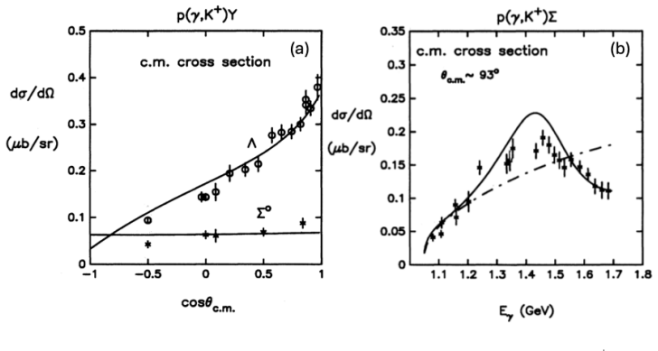
Figure 3.2. Figure 3.2: Representative key early results from KY photoproduction studies. (a) Differential cross section from Cornell (1958) for K+Λ at Elab γ = 980 MeV and 1010 MeV as a function of θ c.m. K . Figure from Ref. [56]. (b) Λ recoil polarization P for exclusive K+Λ as a function of Elab γ for θ c.m. K ≈ 0 ◦ from Cornell (1963) (open squares) [70], Frascati (1964) (open triangles) [71], and CalTech (1967) (solid cir… view at source ↗
Figure 3.3
Figure 3.3. Figure 3.3: Representative key early results from KY electroproduction studies. Differential cross sections for (a) K+Λ and (b) K+Σ0 vs. Q2 for data at an average W of 2.15 GeV selected for θ c.m. K < 25◦. The solid line is a dipole fit to the available data. cos Φ moment analysis of differential cross sections for (c) K+Λ and (d) K+Σ0 to separate σU (= σT + ϵσL), σLT (σI), and σTT (σP) vs. four-momentum transfer sq… view at source ↗
Figure 3.4
Figure 3.4. Figure 3.4: Missing mass MM(e ′K+) spectrum from an early electroproduction experiment showing contributions from the ground state Λ and Σ0 , as well as the hyperon excited states Σ(1385), Λ(1405), and Λ(1520). This spectrum from DESY (1975) shows the total dataset for final analysis with 9885 events. Figure from Ref. [78]. Reprinted with permission from Elsevier. sensitivity of the KY channels to explorations of N … view at source ↗
Figure 3.5
Figure 3.5. Figure 3.5: Schematic drawings of the three large acceptance hadronic physics installations at ELSA: (a) SAPHIR – showing the photon [PITH_FULL_IMAGE:figures/full_fig_p026_3_5.png] view at source ↗
Figure 3.6
Figure 3.6. Figure 3.6: Total cross section for (a) γp → K+Λ and (b) γp → K+Σ0 from SAPHIR (red stars, red triangles) [82, 87], CLAS (blue circles) [88], and the ABBHHM Collaboration (light blue squares) using data collected at DESY [61]. The curves are from the isobar models Kaon-MAID (solid red, dotted red) [89] and Saclay-Lyon (dot-dashed black) [90], as well as from a pure Regge model (dashed blue) [91]. Figures from Ref. [… view at source ↗
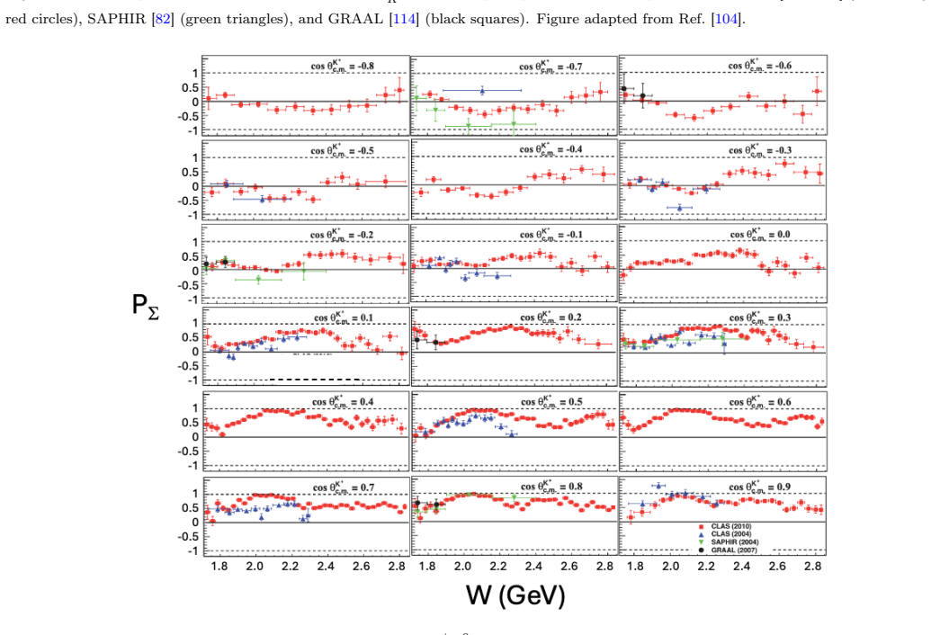
Figure 3.7
Figure 3.7. Figure 3.7: Differential cross section of γp → K+Λ for cos θ c.m. K > 0.90 from BGOOD (black filled circles). Other data shown in the figure are from CLAS (red open triangles, blue open squares) [88, 104], SAPHIR (green open diamonds) [82], and LEPS (orange filled triangle, orange filled squares) [105, 106]. The Regge plus resonance model [107] and isobar models BS1 and BS3 [108, 109] of Skoupil and Bydžovský are th… view at source ↗
Figure 3.8
Figure 3.8. Figure 3.8: Schematic view of the LAGRANGE detector at GRAAL: (1) BGO calorimeter, (2) plastic scintillator barrel, (3) cylindrical [PITH_FULL_IMAGE:figures/full_fig_p029_3_8.png] view at source ↗
Figure 3.9
Figure 3.9. Figure 3.9: Schematic of (a) the LEPS detector at SPring-8 (Figure from Ref. [ [PITH_FULL_IMAGE:figures/full_fig_p030_3_9.png] view at source ↗
Figure 3.10
Figure 3.10. Figure 3.10: Schematic of the experimental layouts at MAMI. (a) Configuration of the electron beam experiments in the A1 area including the [PITH_FULL_IMAGE:figures/full_fig_p032_3_10.png] view at source ↗
Figure 3.11
Figure 3.11. Figure 3.11: Differential cross sections for γn → K0Λ from MAMI A2 (black circles) plotted as a function of cos θ c.m. K for bins in W. The data are compared to results from CLAS (solid magenta and solid blue triangles) [142]. The green curves are a prediction from the partial wave analysis of Ref. [143] and the red line is a linear fit. Figure from Ref. [144] and used with kind permission of The European Physical J… view at source ↗
Figure 3.12
Figure 3.12. Figure 3.12: Differential cross sections for γn → K0Σ0 from MAMI A2 plotted as a function of cos θ c.m. K for bins in W [144]. The blue curve is from the isobar model of Ref. [26] and the red line is a linear fit. Figure from Ref. [144] and used with kind permission of The European Physical Journal (EPJ). 33 [PITH_FULL_IMAGE:figures/full_fig_p033_3_12.png] view at source ↗
Figure 3.13
Figure 3.13. Figure 3.13: (a) Schematic of the Hall A spectrometer setup showing the two identical HRS high resolution spectrometers. In this figure the [PITH_FULL_IMAGE:figures/full_fig_p035_3_13.png] view at source ↗
Figure 3.14
Figure 3.14. Figure 3.14: An example MM(e ′K+) spectrum from a Hall C measurement showing well separated Λ and Σ0 hyperon peaks. The vertical lines define the hyperon masses. This spectrum has been background subtracted to remove accidental coincidences and cryotarget window contributions. Figure from Ref. [160]. 36 [PITH_FULL_IMAGE:figures/full_fig_p036_3_14.png] view at source ↗
Figure 3.15
Figure 3.15. Figure 3.15: Differential cross sections as a function of the transverse virtual photon polarization parameter [PITH_FULL_IMAGE:figures/full_fig_p037_3_15.png] view at source ↗
Figure 3.16
Figure 3.16. Figure 3.16: Charged kaon form factor vs. Q2 from JLab Hall C measurements of σL (red squares and black circles). The dashed black curve shows the monopole form factor distribution [165]; the solid blue line shows the form factor from a Dyson-Schwinger model and the dotted pink curve corresponds to a leading-order pQCD calculation [166]. Figure from Ref. [162]. angles. The final optimized configuration employed a ne… view at source ↗
Figure 3.17
Figure 3.17. Figure 3.17: Schematic of the JLab hypernuclear spectroscopy configuration in Hall C. The setup consists of the HES electron arm, the HKS [PITH_FULL_IMAGE:figures/full_fig_p038_3_17.png] view at source ↗
Figure 3.18
Figure 3.18. Figure 3.18: Binding energy spectra for (a) 12 ΛB and (b) 10 ΛBe from the final JLab Hall C 6-GeV era experiments of the hypernuclear program. The fit functions are shown on each plot. Figures from Refs. [169] (a) and [171] (b). 3.6.2. Hall B – CLAS Photoproduction Program The large acceptance CLAS spectrometer in Hall B [172] was operational in the period from 1997 to 2012. The spectrom￾eter was constructed around … view at source ↗
Figure 3.19
Figure 3.19. Figure 3.19: Schematic view of the CLAS detector with the different subsystems labeled (DC: drift chamber, SC: scintillation counters, CC: [PITH_FULL_IMAGE:figures/full_fig_p039_3_19.png] view at source ↗
Figure 3.20
Figure 3.20. Figure 3.20: Experimental yield distribution in terms of [PITH_FULL_IMAGE:figures/full_fig_p042_3_20.png] view at source ↗
Figure 3.21
Figure 3.21. Figure 3.21: Differential cross sections for K+Λ photoproduction vs. W binned in cos θ c.m. K . The plot includes data from CLAS [88, 104] (open blue triangles, red circles), SAPHIR [82] (open green diamonds), and LEPS [123, 191] (open black circles). Figure adapted from Ref. [104] [PITH_FULL_IMAGE:figures/full_fig_p043_3_21.png] view at source ↗
Figure 3.22
Figure 3.22. Figure 3.22: Differential cross sections for K+Σ0 photoproduction vs. W binned in cos θ c.m. K . The plot includes data from CLAS [88, 176] (blue up-triangles, red squares), SAPHIR [82] (green down-triangles), and LEPS [122] (black circles). Figure adapted from Ref. [176]. 43 [PITH_FULL_IMAGE:figures/full_fig_p043_3_22.png] view at source ↗
Figure 3.23
Figure 3.23. Figure 3.23: Recoil polarization P vs. W binned in cos θ c.m. K for K+Λ photoproduction from a proton from CLAS [104, 175] (blue triangles, red circles), SAPHIR [82] (green triangles), and GRAAL [114] (black squares). Figure adapted from Ref. [104] [PITH_FULL_IMAGE:figures/full_fig_p044_3_23.png] view at source ↗
Figure 3.24
Figure 3.24. Figure 3.24: Recoil polarization P vs. W binned in cos θ c.m. K for K+Σ0 photoproduction from a proton from CLAS [175, 176] (blue up-triangles, red circles), SAPHIR [82] (green down-triangles), and GRAAL [114] (black circles). Figure adapted from Ref. [176]. 44 [PITH_FULL_IMAGE:figures/full_fig_p044_3_24.png] view at source ↗
Figure 3.25
Figure 3.25. Figure 3.25: Cz (top) and Cx (bottom) beam-recoil hyperon transferred polarization for exclusive K+Λ production extracted from the first generation CLAS dataset (red) [179] compared to second-generation CLAS results (black) [180] as a function of W for representative cos θ c.m. K bins as shown. Figure from Ref. [180]. in cos θ c.m. K [181]. Note that these data were taken with a unpolarized liquid-hydrogen target. T… view at source ↗
Figure 3.26
Figure 3.26. Figure 3.26: The energy dependence of the beam asymmetry [PITH_FULL_IMAGE:figures/full_fig_p046_3_26.png] view at source ↗
Figure 3.27
Figure 3.27. Figure 3.27: The energy dependence of the beam asymmetry [PITH_FULL_IMAGE:figures/full_fig_p046_3_27.png] view at source ↗
Figure 3.28
Figure 3.28. Figure 3.28: Comparison of differential cross sections from CLAS data for the [PITH_FULL_IMAGE:figures/full_fig_p047_3_28.png] view at source ↗
Figure 3.29
Figure 3.29. Figure 3.29: Key results from the CLAS Ξ photoproduction analyses. (a) Distribution of the MM(K+K+) events showing the exclusive reaction yields for the ground state Ξ−(1321) and first excited state Ξ−(1530). (b) Total cross section for the ground Ξ and first excited state as a function of W. (c) First measurement of the Ξ−(1321) recoil and beam-recoil hyperon transferred polarization components as a function of pho… view at source ↗
Figure 3.30
Figure 3.30. Figure 3.30: Kinematic coverage of a CLAS 6-GeV KY electroproduction dataset in terms of (a) Q2 (GeV2 ) vs. W (GeV) and (b) cos θ c.m. K vs. Φ. The plots are overlaid with the binning choices from the analysis. Figure from Ref. [224] [PITH_FULL_IMAGE:figures/full_fig_p050_3_30.png] view at source ↗
Figure 3.31
Figure 3.31. Figure 3.31: Kinematics for K+Y electroproduction defining the c.m. angles and coordinate systems used to express the formalism and to present the hyperon polarization components. Here the primed coordinate system is connected to the K+ with the z ′ axis along its direction and the y ′ axis normal to the hadronic reaction plane. The unprimed coordinate system is connected with the virtual photon with the z along alo… view at source ↗
Figure 3.32
Figure 3.32. Figure 3.32: Structure functions σU = σT + ϵσL, σLT, σTT, and σLT′ (nb/sr) from CLAS data for K+Λ production vs. W (GeV) for Ebeam = 5.5 GeV for Q2 = 1.80 GeV2 and cos θ c.m. K values as shown. The error bars represent the statistical uncertainties only. The red curves are from the hadrodynamic KY model of Maxwell [233], the blue curves are from the hybrid RPR-2011 KY model from Ghent [234], and the black curves are… view at source ↗
Figure 3.33
Figure 3.33. Figure 3.33: Structure functions σU = σT + ϵσL, σLT, σTT, and σLT′ (nb/sr) from CLAS data for K+Σ0 production vs. W (GeV) for Ebeam = 5.5 GeV for Q2 = 1.80 GeV2 and cos θ c.m. K values as shown. The error bars represent the statistical uncertainties only. The blue curves are from the hybrid RPR-2007 KY model from Ghent [235] and the black curves are from the GLV Regge model [91]. Figure from Ref. [224]. transverse r… view at source ↗
Figure 3.34
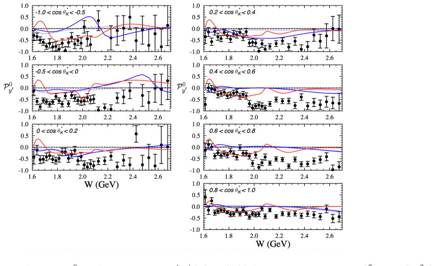
Figure 3.34. Figure 3.34: Recoil hyperon polarization P0 y′ in the reaction ep → e ′K+Λ from CLAS data vs. W at an average Q2 = 1.9 GeV2 for Ebeam = 5.5 GeV and cos θ c.m. K ranges as shown. The error bars represent the statistical uncertainties only. The red curves are from the isobar model of Maxwell [233] and the blue curves are from the hybrid RPR-2011 KY model from Ghent [234]. Figure adapted from Ref. [225]. one gluon exch… view at source ↗
Figure 3.35
Figure 3.35. Figure 3.35: Beam-recoil hyperon transferred polarization components [PITH_FULL_IMAGE:figures/full_fig_p055_3_35.png] view at source ↗
Figure 3.36
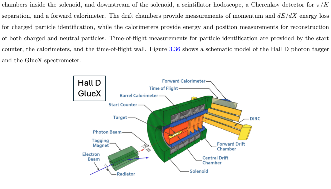
Figure 3.36. Figure 3.36: Model representation of the GlueX tagger hall and spectrometer in Hall D. The detector subsystems are labeled and outlined in [PITH_FULL_IMAGE:figures/full_fig_p059_3_36.png] view at source ↗
Figure 3.37
Figure 3.37. Figure 3.37: The linearly polarized beam spin asymmetry [PITH_FULL_IMAGE:figures/full_fig_p060_3_37.png] view at source ↗
Figure 3.38
Figure 3.38. Figure 3.38: Spin density matrix elements ρ (ρ 0 unpolarized, ρ 1,2 polarized) as a function of four-momentum transfer squared t measured at GlueX for exclusive photoproduction of Λ(1520) [270] compared to predictions from a Regge approach [281] constrained by data from CLAS [188] and LEPS [150, 151] (blue solid) and from LAMP2 (the Large Aperture Magnetic Spectrometer at Daresbury [282]) [68] and SLAC [63] (red das… view at source ↗
Figure 3.39
Figure 3.39. Figure 3.39: Spectroscopy studies at GlueX for various [PITH_FULL_IMAGE:figures/full_fig_p062_3_39.png] view at source ↗
Figure 3.40
Figure 3.40. Figure 3.40: Model representation of the CLAS12 spectrometer in Hall B. The detector subsystems are labeled and outlined in the text. The [PITH_FULL_IMAGE:figures/full_fig_p063_3_40.png] view at source ↗
Figure 3.41
Figure 3.41. Figure 3.41: Kinematic coverage of CLAS12 from data with an 11 GeV electron on a liquid-hydrogen target in terms of [PITH_FULL_IMAGE:figures/full_fig_p064_3_41.png] view at source ↗
Figure 3.42
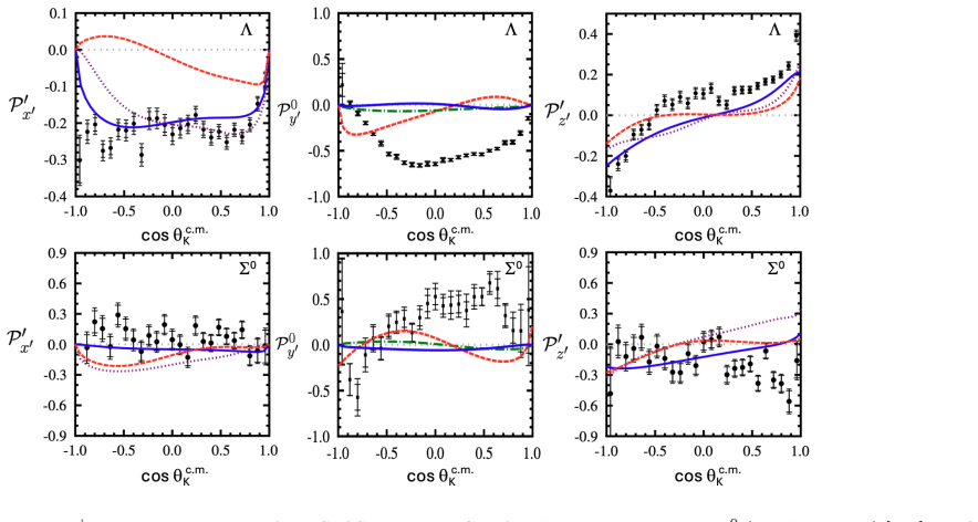
Figure 3.42. Figure 3.42: Representative K+Y polarization results from CLAS12 at 6.535 GeV for the recoil polarization P0 (middle column) [232] and for the beam-recoil transferred polarization P′ (outer columns) [289] with respect to the (x ′ , y′ , z′ ) coordinate system defined in [PITH_FULL_IMAGE:figures/full_fig_p066_3_42.png] view at source ↗
Figure 3.43
Figure 3.43. Figure 3.43: Projections of the kinematic reach and uncertainties of the charged kaon form factor vs. [PITH_FULL_IMAGE:figures/full_fig_p068_3_43.png] view at source ↗
Figure 3.44
Figure 3.44. Figure 3.44: (a) Evolution of the K+Y cross section vs. Q2 (assuming a dipole form factor) to illustrate the kinematic range opened up by the possible energy upgrade of JLab to 22 GeV. This figure shows the rapid fall-off of the cross section at increasing Q2 that must be compensated for with data-taking at higher beam-target luminosities and longer running times. (b) Preliminary simulation results for exclusive KY … view at source ↗
Figure 4.1
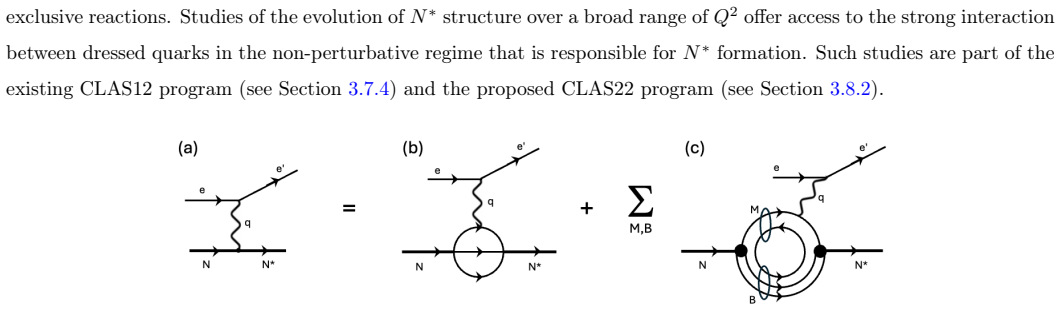
Figure 4.1. Figure 4.1: Schematic representation of the γvN → N∗ electroproduction process. (a) The fully dressed γvNN∗ electrocoupling that determines the N∗ contribution to the resonant part of the meson electroproduction amplitude. (b) The contribution of the three-quark core. (c) The contribution from the meson-baryon cloud, where the sum is over all intermediate meson and baryon states. Figure motivation from Ref. [332]. E… view at source ↗
Figure 5.1
Figure 5.1. Figure 5.1: Quark-flow diagrams for K+ photoproduction in the semi-relativistic quark model (SRQM). Panel (a) shows the direct photon￾induced creation of an ss¯ pair, representing the seagull term, while panels (b), (c), and (d) illustrate indirect production mechanisms corre￾sponding to the s-, u-, and t-channel processes, respectively. Figures adapted from Ref. [10]. required by gauge invariance. To resolve this s… view at source ↗
Figure 5.2
Figure 5.2. Figure 5.2: The CDM predictions for the γp → K+Λ differential cross sections compared with experimental data plotted as a function of cos θ c.m. K (a)-(d) and the photon laboratory energy (e)-(f). The differences between the solid and dashed curves illustrate the sensitivity of the model to a 10% variation in the kaon decay constant fK. Figures from Ref. [351]. The chiral quark model (χQM) of Li [353], developed as … view at source ↗
Figure 5.3
Figure 5.3. Figure 5.3: Total cross sections vs. Elab γ predicted by the chiral quark model compared to the experimental data for the (a) γp → K+Λ and (b) γp → K+Σ0 channels. Figures from Ref. [353]. The χQM was subsequently extended to study KΣ photoproduction in all four isospin channels [356], yielding better overall agreement with the available data than traditional isobar models. It should be emphasized, however, that the … view at source ↗
Figure 5.4
Figure 5.4. Figure 5.4: Comparison of heavy-baryon ChPT predictions with experimental photoproduction data for the total cross sections of (a) [PITH_FULL_IMAGE:figures/full_fig_p079_5_4.png] view at source ↗
Figure 5.5
Figure 5.5. Figure 5.5: The three possible Feynman diagrams for the electromagnetic production of kaons on the nucleon [PITH_FULL_IMAGE:figures/full_fig_p080_5_5.png] view at source ↗
Figure 5.6
Figure 5.6. Figure 5.6: (a) Comparison of the angular dependence of the differential cross section data with the fits of Thom. The resonant states in each fit [PITH_FULL_IMAGE:figures/full_fig_p082_5_6.png] view at source ↗
Figure 5.7
Figure 5.7. Figure 5.7: Comparison between the fits and total cross sections of the [PITH_FULL_IMAGE:figures/full_fig_p083_5_7.png] view at source ↗
Figure 5.8
Figure 5.8. Figure 5.8: (a) Results of the Renard-Renard model for the differential cross section of the [PITH_FULL_IMAGE:figures/full_fig_p084_5_8.png] view at source ↗
Figure 5.9
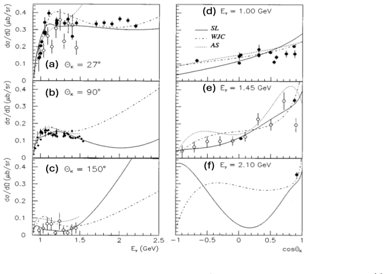
Figure 5.9. Figure 5.9: Predictions of the WJC model for the angular dependence of the differential cross section of the [PITH_FULL_IMAGE:figures/full_fig_p085_5_9.png] view at source ↗
Figure 5.10
Figure 5.10. Figure 5.10: (a) Results of the WJC91 model for the angular distribution of the differential cross section of [PITH_FULL_IMAGE:figures/full_fig_p086_5_10.png] view at source ↗
Figure 5.11
Figure 5.11. Figure 5.11: Prediction of the SL model for the differential cross section of the [PITH_FULL_IMAGE:figures/full_fig_p087_5_11.png] view at source ↗
Figure 5.12
Figure 5.12. Figure 5.12: (a) Prediction of the SL model for the structure function [PITH_FULL_IMAGE:figures/full_fig_p088_5_12.png] view at source ↗
Figure 5.13
Figure 5.13. Figure 5.13: Comparison between the differential cross section data for the [PITH_FULL_IMAGE:figures/full_fig_p089_5_13.png] view at source ↗
Figure 5.14
Figure 5.14. Figure 5.14: Total cross section data for K+Λ photoproduction on the proton as a function of the c.m. energy W. The solid green squares are the SAPHIR data [87], while the open circles show older Aachen-Berlin-Bonn-Hamburg-Heidelberg-München Collaboration data [61]. The dashed blue line displays the model without the N(1960)3/2−. The inclusion of the N(1960)3/2− leads to the model represented by the solid red line. … view at source ↗
Figure 6
Figure 6. Figure 6: The total cross sections up to energy Eγ = 2.1 GeV; lines as in [PITH_FULL_IMAGE:figures/full_fig_p092_6.png] view at source ↗
Figure 5.16
Figure 5.16. Figure 5.16: Energy dependence of the differential cross section of the [PITH_FULL_IMAGE:figures/full_fig_p094_5_16.png] view at source ↗
Figure 5.17
Figure 5.17. Figure 5.17: (a) Comparison between the BS3 model and the differential cross section data for [PITH_FULL_IMAGE:figures/full_fig_p095_5_17.png] view at source ↗
Figure 5.18
Figure 5.18. Figure 5.18: Contributions of the rescattering terms in electromagnetic production of kaons, illustrating the Lippmann-Schwinger equation [PITH_FULL_IMAGE:figures/full_fig_p100_5_18.png] view at source ↗
Figure 5.19
Figure 5.19. Figure 5.19: Samples of differential cross sections for the [PITH_FULL_IMAGE:figures/full_fig_p102_5_19.png] view at source ↗
Figure 5.20
Figure 5.20. Figure 5.20: As in Fig [PITH_FULL_IMAGE:figures/full_fig_p102_5_20.png] view at source ↗
Figure 5.21
Figure 5.21. Figure 5.21: (a) Selected differential cross sections for [PITH_FULL_IMAGE:figures/full_fig_p104_5_21.png] view at source ↗
Figure 5.22
Figure 5.22. Figure 5.22: (a) Comparison of the transferred Λ polarization components P′ x, P′ z , P′ x′ , and P′ z′ with predictions from the JBW DCC model [243] and Kaon-MAID [24]. The shaded bands connect the different solutions denoted by FIT1,...,4 to guide the eye. Predictions from Kaon-Maid are displayed as green dash-dot-dotted lines. The experimental data are from Ref. [289]. (b) Ratio of the longitudinal to transverse … view at source ↗
Figure 5.23
Figure 5.23. Figure 5.23: (a) Real and imaginary parts of the p → N(1440)1/2 + transition form factors at low Q2 , obtained from the JBW DCC model [465] and the ANL-Osaka model [482]. The two error bars at Q2 = 0 indicate the uncertainties of the photoproduction pole solution. (b) Transverse charge density for the p → N(1440)1/2 + transition as a function of the transverse distance b in the xy plane. Figures from Ref. [465]. 5.4… view at source ↗
Figure 5.24
Figure 5.24. Figure 5.24: Comparison of the γp → K+Λ differential cross sections obtained from the Giessen model with experimental data from SAPHIR [82] and CLAS [175]. The solid and dashed curves correspond to fits to the CLAS (C parameter set) and SAPHIR (S parameter set) data, respectively. Figure from Ref. [510]. include a wide range of single- and double-polarization observables, covering the full angular distributions of t… view at source ↗
Figure 5.25
Figure 5.25. Figure 5.25: Sample of the γp → K+Λ differential cross sections vs. cos θ c.m. K for different W bins (as labeled) predicted by the KSU (solid lines) [143] and BnGa 2016 (dashed lines) [516] models. Figures adapted from Ref. [143]. Froissart bound, we refer readers to Ref. [517]. A way to resolve the shortcomings of isobar models was introduced in 1959 by Regge. His idea was to extend the concept of partial wave amp… view at source ↗
Figure 5.26
Figure 5.26. Figure 5.26: The Chew-Frautschi plot for the K(494) and K∗(892) Regge trajectories. The mass of each particle is taken from Ref. [209]. The trajectories satisfy αK(t) = 0.64(t − m2 K) and αK∗ (t) = 1 + 0.85(t − m2 K∗ ). electroproduction reactions at forward angles are dominated by the t-channel K and K∗ Regge exchanges (equivalently, u￾channel exchanges for backward angles). The Regge exchanges were introduced by f… view at source ↗
Figure 5.27
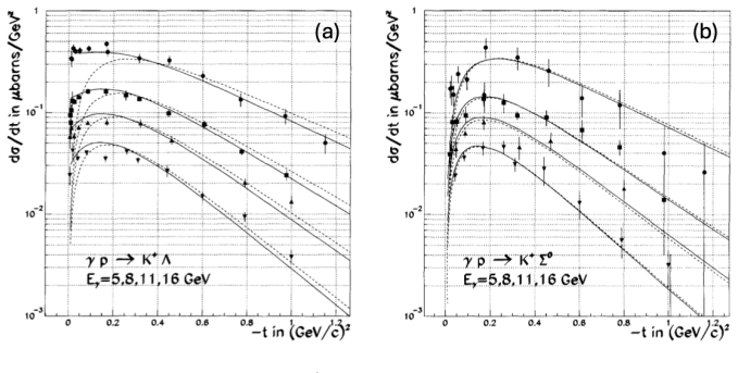
Figure 5.27. Figure 5.27: (a) Differential cross section dσ/dt for the γp → K+Λ reaction for four photon energies as a function of the Mandelstam variable t. The solid curves show the full Reggeized K and K∗ exchanges while the dashed curves show only the contribution from K∗ exchanges. Experimental data from Ref. [62]. (b) Same, but for the γp → K+Σ0 reaction. Figures from Ref. [531]. Reprinted with permission from Elsevier. st… view at source ↗
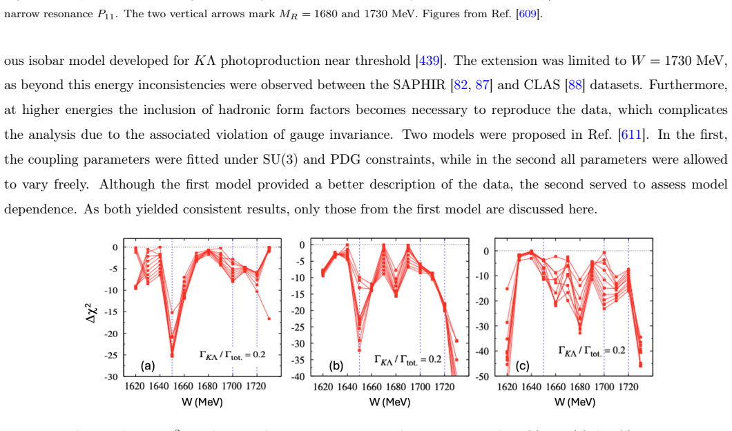
Figure 5.28
Figure 5.28. Figure 5.28: Illustration of the Regge-plus-Resonance approach. The Feynman diagrams in this figure were generated using the [PITH_FULL_IMAGE:figures/full_fig_p113_5_28.png] view at source ↗
Figure 5.29
Figure 5.29. Figure 5.29: (a) Results of the RPR-BS and RPR-BS(pv) models for the differential cross section of the [PITH_FULL_IMAGE:figures/full_fig_p114_5_29.png] view at source ↗
Figure 6.1
Figure 6.1. Figure 6.1: Kaon photoproduction on nuclei within the impulse approximation: (a) kaon photoproduction on the deuteron, [PITH_FULL_IMAGE:figures/full_fig_p116_6_1.png] view at source ↗
Figure 6.2
Figure 6.2. Figure 6.2: Inclusive cross section for kaon photoproduction on the deuteron as a function of kaon laboratory momentum at [PITH_FULL_IMAGE:figures/full_fig_p119_6_2.png] view at source ↗
Figure 6.3
Figure 6.3. Figure 6.3: Comparison of model calculations with experimental data [ [PITH_FULL_IMAGE:figures/full_fig_p120_6_3.png] view at source ↗
Figure 6.4
Figure 6.4. Figure 6.4: (a) Predicted masses and decay amplitudes to the [PITH_FULL_IMAGE:figures/full_fig_p122_6_4.png] view at source ↗
Figure 6.5
Figure 6.5. Figure 6.5: Photon beam spin asymmetry Σ obtained from fits without (dashed blue lines) and with (solid red lines) inclusion of the SAPHIR data from Ref. [87]. Figure from Ref. [89], with color added for clarity. described within a unified algebraic framework. Within this approach, the N(1895)3/2 − state observed in Ref. [89] can be interpreted in terms of several possible configurations. The lowest of these corresp… view at source ↗
Figure 6.6
Figure 6.6. Figure 6.6: (a) Contributions of the background and resonance terms to the [PITH_FULL_IMAGE:figures/full_fig_p124_6_6.png] view at source ↗
Figure 6.7
Figure 6.7. Figure 6.7: (a) Antidecuplet of baryons predicted by the chiral soliton model [ [PITH_FULL_IMAGE:figures/full_fig_p126_6_7.png] view at source ↗
Figure 6.8
Figure 6.8. Figure 6.8: Differential cross sections for η photoproduction on the proton (solid triangles) and neutron (solid circles) as a function of the total c.m. energy, obtained from (a) the photon energy (WB) and (b) reconstructed from the four-vectors of the η meson and the recoiling nucleon (WR). The stars represent the response to a δ function, illustrating the effect of the finite energy resolution. The solid, dash-do… view at source ↗
Figure 6.9
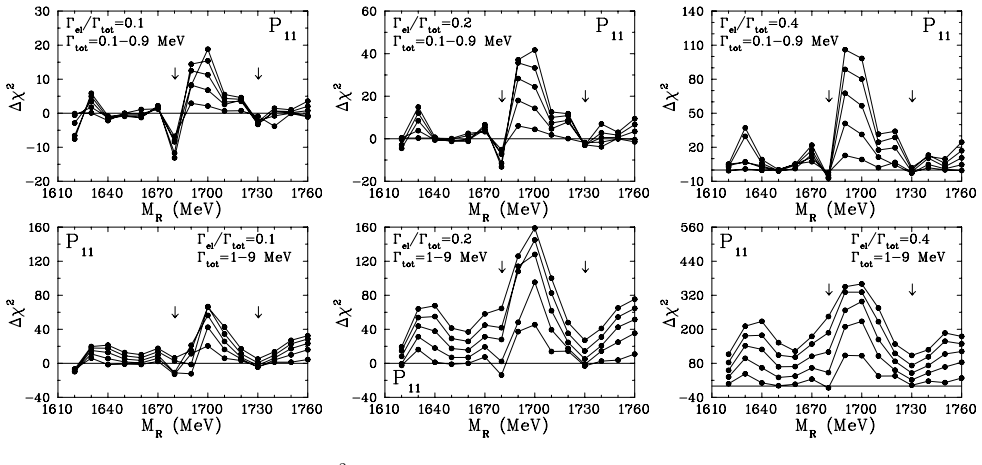
Figure 6.9. Figure 6.9: Dependence of the change of overall χ 2 on the resonance mass MR, relative elastic width Γel/Γtot, and total width Γtot for the narrow resonance P11. The two vertical arrows mark MR = 1680 and 1730 MeV. Figures from Ref. [609]. ous isobar model developed for KΛ photoproduction near threshold [439]. The extension was limited to W = 1730 MeV, as beyond this energy inconsistencies were observed between the … view at source ↗
Figure 6.10
Figure 6.10. Figure 6.10: Change of overall χ 2 as a function of the resonance mass W after the insertion of the (a) P11, (b) S11, (c) P13 resonances in Model 1 for different values of total width Γtot (from 1 to 10 MeV with 1 MeV step). Figures from Ref. [611]. The analysis method followed that used for the πN channel. By scanning the variation of the total χ 2 as a function of the resonance mass W from 1620 to 1730 MeV in 10 M… view at source ↗
Figure 6.11
Figure 6.11. Figure 6.11: (a) Total photoabsorption cross section (solid squares) and helicity-dependent cross-section difference, [PITH_FULL_IMAGE:figures/full_fig_p131_6_11.png] view at source ↗
Figure 6.12
Figure 6.12. Figure 6.12: Total cross sections σtot (solid lines) and −σTT′ (dashed lines) as a function of the photon laboratory energy ν for the six isospin channels of kaon photoproduction. The K0Λ total cross sections are multiplied by 1/2 to fit within the same scale. Figure from Ref. [627]. In spite of the good agreement with the standard GDH integral, contributions from vector-meson photoproduction were not included in Re… view at source ↗
Figure 6.13
Figure 6.13. Figure 6.13: Electromagnetic form factor of the charged kaon as a function of [PITH_FULL_IMAGE:figures/full_fig_p132_6_13.png] view at source ↗
Figure 6.14
Figure 6.14. Figure 6.14: (a) Contribution from the t-channel diagram in pion (kaon) electroproduction. The amplitude is proportional to the propagator 1/(t − m2 ), where m is the pion (kaon) mass, and is enhanced when |t − m2 | is minimized. The electromagnetic form factors Fπ(Q2 ) and FK(Q2 ) describe the meson charge distribution as a function of Q2 , while the hadronic form factor Fh(t) accounts for the extended structure of… view at source ↗
Figure 6.15
Figure 6.15. Figure 6.15: Longitudinal differential cross sections for neutral kaon electroproduction, [PITH_FULL_IMAGE:figures/full_fig_p134_6_15.png] view at source ↗

discussion (0)

Sign in with ORCID, Apple, or X to comment. Anyone can read and Pith papers without signing in.

Reference graph

Works this paper leans on

298 extracted references · 191 canonical work pages

  1. [1]

    Gell-Mann, Y

    M. Gell-Mann, Y. Ne’eman (Eds.), The Eightfold Way, CRC Press, Boca Raton, FL, USA, 2000.doi:10.1201/ 9780429496615

  2. [2]

    D. J. Gross, Asymptotic Freedom, Confinement and QCD, NATO Sci. Ser. B 352 (1996) 75–99.doi:10.1007/ 978-1-4613-1147-8_7

  3. [3]

    Gross, et al., 50 Years of Quantum Chromodynamics, Eur

    F. Gross, et al., 50 Years of Quantum Chromodynamics, Eur. Phys. J. C 83 (2023) 1125.doi:10.1140/epjc/ s10052-023-11949-2

  4. [4]

    A. J. G. Hey, R. L. Kelly, Baryon Spectroscopy, Phys. Rept. 96 (1983) 71.doi:10.1016/0370-1573(83)90114-X

  5. [5]

    D. G. Ireland, E. Pasyuk, I. Strakovsky, Photoproduction Reactions and Non-Strange Baryon Spectroscopy, Prog. Part. Nucl. Phys. 111 (2020) 103752.doi:10.1016/j.ppnp.2019.103752

  6. [6]

    Burkert, G

    V. Burkert, G. Eichmann, E. Klempt, The Impact ofγNandγ ∗NInteractions on our Understanding of Nucleon Excitations, Prog. Part. Nucl. Phys. 146 (2026) 104214.doi:10.1016/j.ppnp.2025.104214

  7. [7]

    Bennhold, T

    C. Bennhold, T. Mart, F. X. Lee, H. Haberzettl, H. Yamamura, K. Miyagawa, W. Gloeckle, S. S. Kamalov, L. Tiator, L. E. Wright, Hypernuclear Physics with Photons, in: Workshop on Hypernuclear Physics with Electromagnetic Probes (HYJLAB99), 1999.arXiv:nucl-th/0011022

  8. [8]

    F. A. Berends, A. Donnachie, D. L. Weaver, Photoproduction and Electroproduction of Pions. 1. Dispersion Relation Theory, Nucl. Phys. B 4 (1967) 1–53.doi:10.1016/0550-3213(67)90196-4

  9. [9]

    B. B. Deo, A. K. Bisoi, Pseudoscalar Versus Pseudovector Interactions in Photoproduction and Electroproduction of Charged Mesons, Phys. Rev. D 9 (1974) 288–295.doi:10.1103/PhysRevD.9.288

  10. [10]

    Mart, Electromagnetic Production of Kaons off the Nucleon and3He, Ph.D

    T. Mart, Electromagnetic Production of Kaons off the Nucleon and3He, Ph.D. thesis, Johannes Gutenberg Uni- versität Mainz (1996)

  11. [11]

    T. Mart, B. Van Der Ventel, Photo- and Electroproduction of the Hypertriton on3He, Phys. Rev. C 78 (2008) 014004.doi:10.1103/PhysRevC.78.014004

  12. [12]

    Dennery, Theory of the Electro- and Photoproduction ofπMesons, Phys

    P. Dennery, Theory of the Electro- and Photoproduction ofπMesons, Phys. Rev. 124 (1961) 2000–2010.doi: 10.1103/PhysRev.124.2000

  13. [13]

    Knöchlein, D

    G. Knöchlein, D. Drechsel, L. Tiator, Photoproduction and Electroproduction ofηMesons, Z. Phys. A 352 (1995) 327–343.doi:10.1007/BF01289506

  14. [14]

    G. F. Chew, M. L. Goldberger, F. E. Low, Y. Nambu, Relativistic Dispersion Relation Approach to Photomeson Production, Phys. Rev. 106 (1957) 1345–1355.doi:10.1103/PhysRev.106.1345

  15. [15]

    Zagury, Photoproduction and Electroproduction of Pions in the Region of theN∗(1238), Phys

    N. Zagury, Photoproduction and Electroproduction of Pions in the Region of theN∗(1238), Phys. Rev. 145 (1966) 1112–1127.doi:10.1103/PhysRev.145.1112

  16. [16]

    Drechsel, L

    D. Drechsel, L. Tiator, Threshold Pion Photoproduction on Nucleons, J. Phys. G 18 (1992) 449–497.doi:10.1088/ 0954-3899/18/3/004. 142

  17. [17]

    R. L. Walker, Phenomenological Analysis of Single Pion Photoproduction, Phys. Rev. 182 (1969) 1729–1748.doi: 10.1103/PhysRev.182.1729

  18. [18]

    N. Levy, W. Majerotto, B. J. Read, Kaon Photoproduction, Nucl. Phys. B 55 (1973) 493–512.doi:10.1016/ 0550-3213(73)90393-3

  19. [19]

    N. Levy, W. Majerotto, B. J. Read, Kaon Electroproduction, Nucl. Phys. B 55 (1973) 513–523.doi:10.1016/ 0550-3213(73)90394-5

  20. [20]

    I. S. Barker, A. Donnachie, J. K. Storrow, Complete Experiments in Pseudoscalar Photoproduction, Nucl. Phys. B 95 (1975) 347–356.doi:10.1016/0550-3213(75)90049-8

  21. [21]

    R. A. Adelseck, B. Saghai, Kaon Photoproduction: Data Consistency, Coupling Constants, and Polarization Ob- servables, Phys. Rev. C 42 (1990) 108–127.doi:10.1103/PhysRevC.42.108

  22. [22]

    Jacob, G

    M. Jacob, G. C. Wick, On the General Theory of Collisions for Particles with Spin, Annals Phys. 7 (1959) 404–428. doi:10.1006/aphy.2000.6022

  23. [23]

    P. J. Bussey, et al., Polarization Parameters in Positive Pion Photoproduction, Nucl. Phys. B 154 (1979) 205–225. doi:10.1016/0550-3213(79)90511-X

  24. [24]

    T. Mart, C. Bennhold, H. Haberzettl, L. Tiator, An Effective Lagrangian Model for Kaon Photo- and Electropro- duction on the Nucleon,https://maid.kph.uni-mainz.de/kaon/, accessed on February 19, 2026

  25. [25]

    Drechsel, O

    D. Drechsel, O. Hanstein, S. S. Kamalov, L. Tiator, A Unitary Isobar Model for Pion Photoproduction and Electro- production on the Proton up to 1 GeV, Nucl. Phys. A 645 (1999) 145–174.doi:10.1016/S0375-9474(98)00572-7

  26. [26]

    Mart, Electromagnetic Production ofKΣon the Nucleon Near Threshold, Phys

    T. Mart, Electromagnetic Production ofKΣon the Nucleon Near Threshold, Phys. Rev. C 90 (6) (2014) 065202. doi:10.1103/PhysRevC.90.065202

  27. [27]

    J. D. Bjorken, S. D. Drell, Relativistic Quantum Mechanics, International Series In Pure and Applied Physics, McGraw-Hill, New York, 1965

  28. [28]

    Halzen, A

    F. Halzen, A. D. Martin, Quarks and Leptons: An Introductory Course in Modern Particle Physics, John Wiley & Sons, New York, 1984

  29. [29]

    Donnachie, Photo and Electroproduction Processes, Vol

    A. Donnachie, Photo and Electroproduction Processes, Vol. 5, Academic Press, New York, 1972, pp. 1–185

  30. [30]

    J. J. de Swart, The Octet Model and its Clebsch-Gordan Coefficients, Rev. Mod. Phys. 35 (1963) 916–939, [Erratum: Rev. Mod. Phys. 37, 326–326 (1965)].doi:10.1103/RevModPhys.35.916

  31. [31]

    J. F. Donoghue, B. R. Holstein, Evidence for SU(3) Breaking in Cabibbo Fits of Semileptonic Hyperon Decay, Phys. Rev. D 25 (1982) 2015.doi:10.1103/PhysRevD.25.2015

  32. [32]

    T. Mart, C. Bennhold, C. E. Hyde-Wright, Constraints on Coupling Constants Through ChargedΣPhotoproduc- tion, Phys. Rev. C 51 (1995) R1074–R1077.doi:10.1103/PhysRevC.51.R1074

  33. [33]

    Haberzettl, C

    H. Haberzettl, C. Bennhold, T. Mart, T. Feuster, Gauge-Invariant Tree-Level Photoproduction Amplitudes with Form Factors, Phys. Rev. C 58 (1) (1998) R40–R44.doi:10.1103/PhysRevC.58.R40. 143

  34. [34]

    Haberzettl, C

    H. Haberzettl, C. Bennhold, T. Mart, Gauge-Invariant Description of Photoproduction and Electroproduction of Mesons with Extended Nucleons Applied to Kaon Production, Nucl. Phys. A 684 (2001) 475–477.doi:10.1016/ S0375-9474(01)00510-3

  35. [35]

    Haberzettl, K

    H. Haberzettl, K. Nakayama, S. Krewald, Gauge-Invariant Approach to Meson Photoproduction Including the Final-State Interaction, Phys. Rev. C 74 (2006) 045202.doi:10.1103/PhysRevC.74.045202

  36. [36]

    Haberzettl, Gauge Invariance of Meson Photo- and Electroproduction Currents Revisited, Phys

    H. Haberzettl, Gauge Invariance of Meson Photo- and Electroproduction Currents Revisited, Phys. Rev. D 104 (5) (2021) 056001.doi:10.1103/PhysRevD.104.056001

  37. [37]

    Ohta, Electromagnetic Interactions of Extended Nucleons, Phys

    K. Ohta, Electromagnetic Interactions of Extended Nucleons, Phys. Rev. C 40 (1989) 1335–1346.doi:10.1103/ PhysRevC.40.1335

  38. [38]

    Haberzettl, Gauge Invariant Theory of Pion Photoproduction with Dressed Hadrons, Phys

    H. Haberzettl, Gauge Invariant Theory of Pion Photoproduction with Dressed Hadrons, Phys. Rev. C 56 (1997) 2041–2058.doi:10.1103/PhysRevC.56.2041

  39. [39]

    R. M. Davidson, R. Workman, Form-Factors and Photoproduction Amplitudes, Phys. Rev. C 63 (2001) 025210. doi:10.1103/PhysRevC.63.025210

  40. [40]

    J. F. Donoghue, E. Golowich, B. R. Holstein, Dynamics of the Standard Model: Second edition, Cambridge Uni- versity Press, 2022.doi:10.1017/9781009291033

  41. [41]

    McAleer, A Measurement of the Recoil Polarization of ElectroproducedΛ(1116), Ph.D

    S. McAleer, A Measurement of the Recoil Polarization of ElectroproducedΛ(1116), Ph.D. thesis, Florida State U. (2002).doi:10.2172/824912

  42. [42]

    Crede, J

    V. Crede, J. Yelton, 70 Years of Hyperon Spectroscopy: A Review of StrangeΞ,ΩBaryons, and the Spectrum of Charmed and Bottom Baryons, Rept. Prog. Phys. 87 (10) (2024) 106301.doi:10.1088/1361-6633/ad7610

  43. [43]

    G. D. Rochester, C. C. Butler, Evidence for the Existence of New Unstable Elementary Particles, Nature 160 (1947) 855–857.doi:10.1038/160855a0

  44. [44]

    V. D. Hopper, S. Biswas, Evidence Concerning the Existence of the New Unstable Elementary Neutral Particle, Phys. Rev. 80 (1950) 1099–1100.doi:10.1103/PhysRev.80.1099

  45. [45]

    C. M. York, R. B. Leighton, E. K. Bjornerud, Direct Experimental Evidence for the Existence of a Heavy Positive VParticle, Phys. Rev. 90 (1953) 167–168.doi:10.1103/PhysRev.90.167

  46. [46]

    Armenteros, K

    R. Armenteros, K. Barker, C. Butler, A. Cachon, C. York, LVI. The Properties of ChargedV-Particles, The London, Edinburgh, and Dublin Philosophical Magazine and Journal of Science 43 (341) (1952) 597–611.doi: 10.1080/14786440608520216

  47. [47]

    Anderson, et al., Cascade Decay ofVParticles, Phys

    C. Anderson, et al., Cascade Decay ofVParticles, Phys. Rev. 92 (1953) 1089

  48. [48]

    W. D. Walker,Λ0 −θ 0 Production inπ−pCollisions at 1 BeV, Phys. Rev. 98 (1955) 1407–1410.doi:10.1103/ PhysRev.98.1407

  49. [49]

    Gell-Mann, A

    M. Gell-Mann, A. Pais, Behavior of Neutral Particles Under Charge Conjugation, Phys. Rev. 97 (1955) 1387–1389. doi:10.1103/PhysRev.97.1387. 144

  50. [50]

    Venanzoni, Discovery of Strangeness (1943-1959); Presented as a seminar to the Muon Group, Liverpool - Apr

    G. Venanzoni, Discovery of Strangeness (1943-1959); Presented as a seminar to the Muon Group, Liverpool - Apr. 29, 2024,https://indico.ph.liv.ac.uk/event/1621/(2024)

  51. [51]

    G. T. Mulholland, G. G. Harigel, Liquid Hydrogen: Target, Detector, AIP Conf. Proc. 710 (2004) 16–26.doi: 10.1063/1.1774662

  52. [52]

    P. L. Donoho, R. L. Walker, Photoproduction ofK+ Mesons in Hydrogen, Phys. Rev. 112 (1958) 981–986.doi: 10.1103/PhysRev.112.981

  53. [53]

    D. E. Groom, J. H. Marshall,ΛPolarization at 90◦ inK +ΛPhotoproduction, Phys. Rev. 159 (1967) 1213–1219. doi:10.1103/PhysRev.159.1213

  54. [54]

    C. J. Bebek, A. Browman, C. N. Brown, K. M. Hanson, R. V. Kline, D. Larson, F. M. Pipkin, S. W. Raither, A. Silverman, L. K. Sisterson, Scalar-Transverse Separation of ElectroproducedK +ΛandK +Σ0 Final States, Phys. Rev. D 15 (1977) 3082.doi:10.1103/PhysRevD.15.3082

  55. [55]

    Abe, et al., Inclusive Photoproduction of Strange Baryons at 20 GeV, Phys

    K. Abe, et al., Inclusive Photoproduction of Strange Baryons at 20 GeV, Phys. Rev. D 32 (1985) 2869–2882. doi:10.1103/PhysRevD.32.2869

  56. [56]

    B. D. McDaniel, A. Silverman, R. R. Wilson, G. Cortellessa, Photoproduction ofKMesons, Phys. Rev. Lett. 1 (1958) 109–111.doi:10.1103/PhysRevLett.1.109

  57. [57]

    B. D. McDaniel, A. Silverman, R. R. Wilson, G. Cortellessa, Photoproduction ofK+ Mesons, Phys. Rev. 115 (1959) 1039–1048.doi:10.1103/PhysRev.115.1039

  58. [58]

    R.L.Anderson, E.Gabathuler, D.Jones, B.D.McDaniel, A.J.Sadoff, PhotoproductionofK + MesonsinHydrogen, Phys. Rev. Lett. 9 (1962) 131–133.doi:10.1103/PhysRevLett.9.131

  59. [59]

    C. W. Peck,K+ΛPhotoproduction from Hydrogen at 1200 MeV, Phys. Rev. 135 (1964) B830–B838.doi:10.1103/ PhysRev.135.B830

  60. [60]

    Erbe, et al., Photoproduction of Strange Particles at Energies up to 5.8 GeV, Nuovo Cim

    R. Erbe, et al., Photoproduction of Strange Particles at Energies up to 5.8 GeV, Nuovo Cim. A 49 (1967) 504. doi:10.1393/ncc/i2024-24208-7

  61. [61]

    Erbe, et al., Multipion and Strange-Particle Photoproduction on Protons at Energies up to 5.8 GeV, Phys

    R. Erbe, et al., Multipion and Strange-Particle Photoproduction on Protons at Energies up to 5.8 GeV, Phys. Rev. 188 (1969) 2060–2077.doi:10.1103/PhysRev.188.2060

  62. [62]

    Boyarski, F

    A. Boyarski, F. Bulos, W. Busza, R. E. Diebold, S. D. Ecklund, G. E. Fischer, Y. Murata, J. R. Rees, B. Richter, W. S. C. Williams, Photoproduction ofK+ΛandK +Σ0 from Hydrogen from 5 GeV to 16 GeV, Phys. Rev. Lett. 22 (1969) 1131–1133.doi:10.1103/PhysRevLett.22.1131

  63. [63]

    Boyarski, R

    A. Boyarski, R. E. Diebold, S. D. Ecklund, G. E. Fischer, Y. Murata, B. Richter, M. Sands, Photoproduction ofK+ Hyperon from Hydrogen and Deuterium at 11 GeV, Phys. Lett. B 34 (1971) 547–550.doi:10.1016/0370-2693(71) 90677-0

  64. [64]

    R. L. Anderson, D. Gustavson, D. Ritson, G. A. Weitsch, H. J. Halpern, R. Prepost, D. H. Tompkins, D. E. Wiser, Measurements of Exclusive Photoproduction Processes at Large Values oftandufrom 4 GeV to 7.5 GeV, Phys. Rev. D 14 (1976) 679.doi:10.1103/PhysRevD.14.679. 145

  65. [65]

    Abe, et al., Inclusive Photoproduction of Neutral Strange Particles at 20 GeV, Phys

    K. Abe, et al., Inclusive Photoproduction of Neutral Strange Particles at 20 GeV, Phys. Rev. D 29 (1984) 1877. doi:10.1103/PhysRevD.29.1877

  66. [66]

    Bleckmann, S

    A. Bleckmann, S. Herda, U. Opara, W. Schulz, W. J. Schwille, H. Urbahn, Photoproduction ofK+ΛandK +Σ0 from Hydrogen Between 1.3 and 1.45 GeV, Z. Phys. 239 (1970) 1–15.doi:10.1007/BF01408507

  67. [67]

    Feller, D

    P. Feller, D. Menze, U. Opara, W. Schulz, W. J. Schwille, Photoproduction ofK+Λ0 andK +Σ0 from Hydrogen at Constant Momentum TransfertBetween 1.05 and 2.2 GeV, Nucl. Phys. B 39 (1972) 413–420.doi:10.1016/ 0550-3213(72)90379-3

  68. [68]

    D. P. Barber, et al., Strangeness Exchange in the Photoproduction ofK+Λ(1520)Between 2.8 GeV and 4.8 GeV, Z. Phys. C 7 (1980) 17.doi:10.1007/BF01577315

  69. [69]

    B. D. McDaniel, P. Joos, D. McLeod, S. Richert, D. Zipoy, Polarization ofΛ0 from Photoproduction in Hydrogen, Phys. Rev. Lett. 4 (1960) 33–35.doi:10.1103/PhysRevLett.4.33

  70. [70]

    H. Thom, E. Gabathuler, D. Jones, B. D. McDaniel, W. M. Woodward, Polarization ofΛHyperons from Photo- production in Hydrogen, Phys. Rev. Lett. 11 (1963) 433–435.doi:10.1103/PhysRevLett.11.433

  71. [71]

    Borgia, M

    B. Borgia, M. Grilli, P. Joos, L. Mezzetti, M. Nigro, E. Schiavuta, F. Villa,Λ0 Polarization from the Reaction γ+p→K ++Λ0 in theEnergy Range 950–1050MeV, Nuovo Cim. 32(1) (1964)218–223.doi:10.1007/BF02732605

  72. [72]

    Grilli, L

    M. Grilli, L. Mezzetti, M. Nigro, E. Schiavuta,Λ0-Polarization from the Reactionγ+p→Λ 0 +K + in the Energy Range (950÷1050) MeV, Nuovo Cim. 38 (4) (1965) 1467–1488.doi:10.1007/BF02750071

  73. [73]

    R. Haas, T. Miczaika, U. Opara, K. Quabach, W. J. Schwille, Measurement of the Polarization of theΛ0 in the Reactionγp→K +Λ0 in the Resonance Region, Nucl. Phys. B 137 (1978) 261–268.doi:10.1016/0550-3213(78) 90519-9

  74. [74]

    K. H. Althoff, et al., Photoproduction ofK+Λ0 on Polarized Protons, Nucl. Phys. B 137 (1978) 269–275.doi: 10.1016/0550-3213(78)90520-5

  75. [75]

    C. N. Brown, et al., Coincidence Measurements of SingleK+ Electroproduction, Phys. Rev. Lett. 28 (1972) 1086– 1089.doi:10.1103/PhysRevLett.28.1086

  76. [76]

    C. J. Bebek, et al., Electroproduction ofK+ Mesons in the Forward Direction, Phys. Rev. Lett. 32 (1974) 21–24. doi:10.1103/PhysRevLett.32.21

  77. [77]

    C. J. Bebek, C. N. Brown, P. Bucksbaum, M. Herzlinger, S. D. Holmes, C. A. Lichtenstein, F. M. Pipkin, S. W. Raither, L. K. Sisterson, Electroproduction ofK+ Mesons Along the Virtual Photon Direction, Phys. Rev. D 15 (1977) 594.doi:10.1103/PhysRevD.15.594

  78. [78]

    Azemoon, I

    T. Azemoon, I. Dammann, C. Driver, D. Luke, G. Specht, K. Heinloth, H. Ackermann, E. Ganssauge, F. Janata, D. Schmidt, Production of Hyperons by Virtual Photons, Nucl. Phys. B 95 (1975) 77–97.doi:10.1016/ 0550-3213(75)90481-2. 146

  79. [79]

    Brauel, T

    P. Brauel, T. Canzler, D. Cords, R. Felst, G. Grindhammer, M. Helm, W. D. Kollmann, H. Krehbiel, M. Schadlich, Electroproduction ofπ +n,π −pandK +Λ,K +Σ0 Final States Above the Resonance Region, Z. Phys. C 3 (1979) 101.doi:10.1007/BF01443698

  80. [80]

    Gourdin, J

    M. Gourdin, J. Dufour, Photoproduction of Strange Particles, Il Nuovo Cimento (1955-1965) 27 (6) (1963) 1410– 1430.doi:10.1007/BF02785636

Showing first 80 references.