REVIEW 4 major objections 4 minor 248 references
This paper argues that few-GeV electron and positron beams can measure tiny charged-current weak processes off protons, and that the Q2-shape of those reactions provides a clean, nuclear-model-free route to the long-disputed axial dipole ma
Reviewed by Pith at T0; open to challenge. T0 means a machine referee read the full paper against a public rubric. the ladder, T0–T4 →
T0 review · deepseek-v4-flash
2026-08-02 04:56 UTC pith:GU6XGCWH
load-bearing objection A competent, honest review-style benchmark paper; the QE numbers are usable for the stated inputs, but the 'determine the axial dipole mass' promise is contingent on the dipole ansatz the authors themselves show to be questionable. the 4 major comments →
Weak charged current induced electron and positron scattering off proton at JLab and MAMI energies
The pith
A machine-rendered reading of the paper's core claim, the machinery that carries it, and where it could break.
Core claim
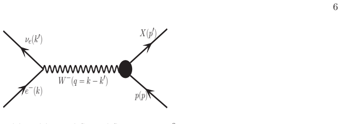
Working in the standard V-A framework, with vector and axial form factors constrained by CVC, PCAC, and SU(3), the paper computes total and differential cross sections plus target spin asymmetries and final-baryon polarizations for e-p -> nu_e + n/Lambda/Sigma0, along with resonance and meson channels. Its central claim is that the Q2 dependence of these observables is sharply sensitive to the axial-vector form factor g1(Q2), while being only mildly sensitive to the weak-electric form factor g2; in particular, the dipole with MA=1.026 GeV, z-expansion fits, and lattice-based g1 differ by 20-45% in dsigma/dQ2. The paper therefore proposes the electron-scattering channel as a new, independent
What carries the argument
The axial-vector form factor g1(Q2), parametrized as gA(0)(1+Q2/MA^2)^-2, together with covariant density-matrix spin formalisms for target asymmetries and final-baryon polarizations; these convert W-exchange amplitudes into Q2-dependent observables whose shape distinguishes between parametrizations of the axial form factor.
Load-bearing premise
The entire benchmark program assumes g1(Q2) is a dipole with MA=1.026 GeV; if the actual axial form factor has a different shape, all quoted cross-section benchmarks and the proposed MA extraction shift by tens of percent.
What would settle it
Measure dsigma/dQ2 for e-p -> nu_e n at E_e about 1.1 GeV over Q2=0-1.4 GeV2. If the normalized Q2 shape matches the z-expansion or lattice parametrizations rather than the MA=1.026 dipole across the 20-45% differences shown here, the paper's default benchmark is falsified.
If this is right
- At the proposed 2.2 GeV, 100 microA, 500 h setup, roughly 10^6 events are expected, making the weak charged-current channel measurable despite its tiny cross section.
- The Q2 shape of dsigma/dQ2 for e-p -> nu_e n discriminates dipole, z-expansion, and lattice g1 at the 20-45% level, allowing MA to be extracted without nuclear-target uncertainties.
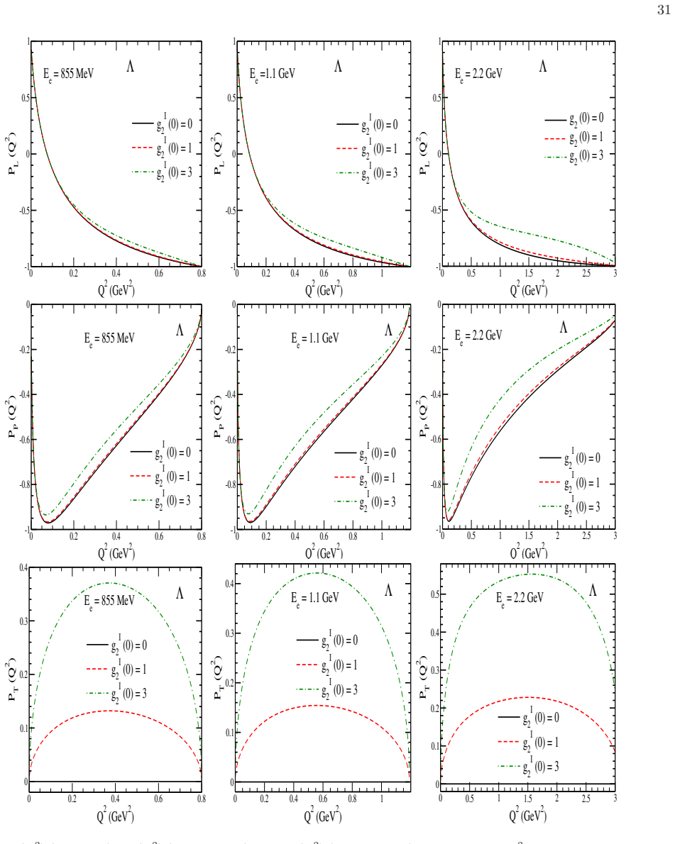
- Final-baryon transverse polarization PT is predicted to vanish under T-invariance and grow with Im[g2(0)], giving a direct test of T-violation.
- For Delta(1232) production, electron and positron beams probe the axial N-Delta transition form factors while avoiding pion-background uncertainties common in neutrino experiments.
- Polarization and asymmetry observables are largely insensitive to MA, so they provide independent cross-checks on the axial sector.
Where Pith is reading between the lines
- If the true axial form factor is not dipole, the extracted MA will be an effective parameter tied to the assumed ansatz; comparing dipole and z-expansion extractions could reveal the underlying shape of g1(Q2).
- Electron-positron comparisons could isolate vector/axial interference terms, potentially separating g1 from g2 more cleanly than either beam alone.
- A multi-energy run across 0.855, 1.1, and 2.2 GeV would map the Q2 shape over different kinematic ranges and test the predicted energy dependence of the MA sensitivity.
- The same formalism can be extended to inelastic channels and nuclear targets, turning these benchmarks into inputs for neutrino-nucleus event generators.
Editorial analysis
A structured set of objections, weighed in public.
Referee Report
Summary. This paper presents a comprehensive theoretical study of charged-current weak processes induced by electrons and positrons on protons at JLab/MAMI energies. The core content is a set of calculations for the quasielastic channels e⁻p→νₑn/Λ/Σ⁰, including total and differential cross sections, target spin asymmetries, and final-baryon polarization observables, with and without time-reversal violation. These are complemented by calculations of Δ(1232), P₁₁(1440), and S₁₁(1535) resonance excitation, η and K/Λ production, and associated strange-particle production. The manuscript claims that these results provide essential theoretical benchmarks for upcoming JLab/MAMI experiments and, in particular, that the quasielastic channel offers an independent way to determine the axial dipole mass M_A and to test G- and T-invariance. The calculations use a standard formalism: leptonic and hadronic tensors, CVC/SU(3) for vector form factors, a dipole axial form factor as the default, and external parametrizations (Bradford electromagnetic form factors, Meyer z-expansion fits, lattice and phenomenological axial inputs).
Significance. If the central claims are taken at face value, the paper would be a valuable reference for a future experimental program: it maps out many observables across a wide kinematic range, identifies channels with significant sensitivity to the axial-vector sector and to second-class currents, and provides a convenient summary of the relevant form-factor inputs. The quasielastic part is internally consistent and builds on standard, well-tested weak-interaction formalism. The paper also gives quantitative sensitivity studies for M_A, g₂(0), C₅ᴬ(0), and alternative g₁(Q²) parametrizations, which is useful for experimental planning. However, the headline claim that the kinematics offers a unique opportunity to determine M_A is load-bearing and, as discussed below, is not supported once the dipole-shape assumption is relaxed; the manuscript itself shows that alternative g₁(Q²) forms change the predictions by tens of percent. The resonance benchmarks are also strongly W_max-dependent. The value of the paper lies more in the systematic calculation machinery and the explicit sensitivity maps than in the specific benchmark numbers, which should be reframed accordingly.
major comments (4)
- [§II.A.1(d), Eq. (28), Figs. 2, 4-6] The central claim of an independent determination of the axial dipole mass M_A rests on the dipole ansatz g₁(Q²)=g_A(0)(1+Q²/M_A²)⁻² with M_A=1.026 GeV. The manuscript itself shows this assumption is not neutral: Fig. 2 shows the combined MINERvA+LQCD z-expansion fit exceeds the dipole by ~30% over the full Q² range, and Fig. 6 shows dσ/dQ² changes by 20-45% at Q²=1 GeV² (about 80% for the Chen-Roberts lattice form). The text also notes that M_A≈1.3-1.35 GeV within the dipole reproduces these alternative parameterizations. Therefore an 'extracted M_A' from these observables is an effective parameter that depends on the assumed functional shape and on the fitted Q² range. To support the stated opportunity claim, the paper should (i) explicitly frame M_A as defined within the dipole ansatz, and (ii) provide a quantitative analysis of how well the proposed JLab/MAMI setup can distinguish th
- [§III.B.5, Figs. 50-51] The resonance cross sections are not robust benchmarks because they depend strongly on the arbitrary choice of W_max. For P₁₁(1440), increasing W_max from 1.4 GeV to ~1.6 GeV raises σ(Eₑ) by about 65% at 1 GeV and ~100% at 2 GeV; for S₁₁(1535), dσ/dQ² in the peak region changes by ~70% when W_max is varied from 1.7 to 1.5 GeV. The manuscript does not provide a physical criterion for choosing W_max or a range of predictions covering this uncertainty. At minimum, the reported cross sections should be accompanied by a W_max-uncertainty band, and the text should state that the resonance-channel benchmarks are only indicative, not quantitative predictions. This is a load-bearing issue because the resonance sections are presented as part of the same 'essential theoretical benchmark' deliverable.
- [§II.C.2, Eq. (51), Figs. 14,17,28,31,40,43] The T-violation predictions scan the free parameter Im g₂(0) over 0-3 (or 1-3) with essentially no experimental input. Since P_T(Q²) is linear in Im g₂(0), the paper is effectively offering a proportionality curve, not a falsifiable prediction. The statement that an experimental observation of P_T 'can be used to probe T-noninvariance' requires either (i) a concrete sensitivity analysis for the proposed JLab/MAMI luminosities, including expected statistical and systematic uncertainties on P_T, or (ii) an explicit statement that the results are templates to be used once an experimental limit on P_T exists. As written, the prominence given to these T-violation predictions exceeds what the current input information justifies.
- [§II.D.1, Fig. 4 (right), §II.D.4, Fig. 18] The total-cross-section correlation plots for g₂^R(0) versus M_A (Figs. 5 and 19) show that for the Λ channel, positive and negative values of g₂^R(0) shift σ(Eₑ) by comparable amounts to M_A variations. The text acknowledges that a nonzero g₂^R(0) can bias the extraction of M_A. This degeneracy is not quantified in terms of a fit or a covariance analysis. Given that the paper aims to provide benchmarks for extracting M_A, the degeneracy between g₂(0) and M_A should be included in the extraction discussion, otherwise the M_A-determination claim is incomplete even within the dipole assumption.
minor comments (4)
- [Introduction] Typo: 'felicitated' should read 'facilitated'. Also, several captions label positron processes as e⁺+p→νₑ+Δ⁺⁺ (e.g., Figs. 47-49) but the final-state neutrino should be \barνₑ; similarly Fig. 51 shows 'e⁺+p→νₑ+N⋆(1535)' although the text discusses electron-induced excitation.
- [Table IV and Section II.A.1] The notation alternates between 'Λ0' and 'Λ' and 'Σ⁰'/'Σ0'; the table header uses 'Λ0' while the text uses 'Λ'. Please unify the notation.
- [§II.A.1(d), Fig. 2] The z-expansion coefficients in Table V are quoted to many digits but no corresponding uncertainties or covariance matrix are given. Since the paper emphasizes sensitivity to different g₁ forms, the reader cannot assess whether the differences between fits are statistically significant. Adding uncertainties would increase the usefulness of these benchmark calculations.
- [§III.B.5, Figs. 50-51] The captions say 'Lines and points have the same meaning as in Fig. 50' but the legends are not fully described in the captions. Please spell out the line styles for each W_max choice in the captions or in the figures themselves.
Circularity Check
No significant circularity: the paper's observables are explicit functions of externally anchored form-factor inputs, and the MA-determination claim is a proposed experimental extraction, not a fitted prediction.
full rationale
The derivation chain is a standard weak-interaction calculation: Eq. (8) gives dσ/dQ² directly in terms of the leptonic and hadronic tensors, with the hadronic current built from vector form factors (Bradford et al.), the axial form factor g1(Q²) taken as input — Eq. (28), the dipole with MA = 1.026 GeV, or z-expansion/lattice alternatives — Eq. (32) for g2(Q²), and SU(3) coefficients for the strangeness-changing channels. The computed cross sections, asymmetries, and polarizations are explicit functions of these inputs; no quantity is fitted to a subset of the presented observables and then renamed as a prediction. The abstract's claim of 'alternative ways to determine the axial dipole mass' is a proposal for future experimental extraction, not a claim that this paper itself determines MA from its own outputs. The paper's own Figs. 2 and 6 quantify the dependence on the g1 parametrization and on MA; this is model dependence and caveat, not circularity. Self-citations occur for the covariant density-matrix formalism and for resonance helicity/cut-off parameters fitted in earlier work to external CLAS photoproduction data; these are methodology citations or externally anchored fits, not a self-referential chain that assumes the present benchmark results. Thus no circular step satisfying the quoted-evidence standard can be identified.
Axiom & Free-Parameter Ledger
free parameters (11)
- MA (axial dipole mass) =
1.026 GeV (world average [11]); varied to 1.35 GeV
- M2 (dipole mass of weak electric form factor g2) =
1.026 GeV (M2 = MA)
- g2R(0)/g2I(0) (second-class current strength) =
scanned: real ±2 (n), ±3 (Λ, Σ⁰); imaginary 0-3
- x1, x2 (SU(3) axial ratios) =
x1 = 0.364; x2 assumed constant
- CA5(0) (N-Δ axial coupling) =
1.2 (GT relation with fπ=0.97mπ, gΔNπ=28.6)
- z-expansion coefficients a0-a6 =
Table V (MINERvA H, LQCD, deuterium, combined)
- Helicity amplitude parameters Aα(0), a1, b1 =
Tables VIII & X (fitted to CLAS electroproduction)
- Strong form-factor cut-offs ΛB = ΛR =
0.75 GeV (proton), 0.72 GeV (neutron)
- CA3/CA4 parametrization constants =
a3=-4.61, b3=2.8 GeV², MA3=1.67 GeV; x3=1, x4=0.74, MAS=1 GeV
- Wmax (invariant-mass upper cut) =
1.4 GeV (P11), 1.5 GeV (S11), 1.8 GeV (η), 1.4 GeV (Δ)
- α (form-factor scale in Dl(x)) =
400 MeV
axioms (8)
- domain assumption CVC hypothesis: f3 = 0 and weak vector form factors equal electromagnetic ones via isospin
- domain assumption PCAC + pion/kaon pole dominance
- domain assumption SU(3) octet symmetry for ΔS=1 transitions with Q²-independent x1,2
- domain assumption G-invariance (absence of second-class currents) in the baseline set: f3 = g2 = 0
- domain assumption T-invariance: all form factors real
- ad hoc to paper Dipole ansatz for g1(Q²) (Eq. 28) and g2 (Eq. 32)
- standard math Rarita-Schwinger formalism for spin-3/2 with off-shell ambiguities accepted
- domain assumption Bradford et al. electromagnetic form factors
read the original abstract
The development of next-generation, high-luminosity, and high-precision charged lepton beam facilities at JLab and MAMI has opened, in recent years, a new frontier in the exploration of weak interaction processes induced by electrons and positrons in the neutral current sector, which can also be used to study weak interaction processes induced by charged currents. In particular, these processes in the intermediate energy regime, spanning from a few hundred MeV to a few GeV, play a crucial role in understanding electroweak dynamics, nucleon structure, and hadronic response functions. This review presents a comprehensive theoretical study of weak charged-current interactions of electrons and positrons with free protons, encompassing quasielastic scattering in both the strangeness conserving and strangeness changing channels, together with inelastic production of the $P_{33}$(1232), $P_{11}$(1440), $S_{11}$(1535) resonances, $\eta$ and $K$ mesons, and associated production of strange particles. We analyse differential and total cross sections, polarization observables of the final baryons, and spin asymmetries of the proton target, demonstrating their sensitivity to the underlying weak interaction dynamics and to possible second class currents, thereby enabling stringent tests of G- and T- invariance. The explored kinematic region also offers a unique and independent opportunity to constrain the axial vector sector of the weak interaction, and it provides a discussion of alternative ways to determine the axial dipole mass in the quasielastic scattering region, a fundamental parameter that is in debate for nearly two decades. It also focuses on the study of the axial-vector form factors associated with the excitation of the $P_{33}(1232)$ resonance in a manner that is free from the uncertainties inherent in their determination from studies of (anti)neutrino-induced weak processes.
Figures






Reference graph
Works this paper leans on
-
[1]
Nonresonant contribution: The expression for the hadronic current jµ corresponding to the various nonresonant diagrams for electron and positron induced single kaon production, as depicted in Fig. 57, are o btained using the nonlinear sigma model discussed 71 (A) W (q) N (p) Λ , Σ(p + q) N (p′) K(pK) (B) W (q) N (p) N (p′) K(pK) π, η(p − p′) (C) W (q) N (...
-
[2]
(142), with Λ R being determined by fitting the experimental photoproduction data [221] and the best fit for spin 1 2 resonances is obtained as Λ R = 1 GeV [234]
Spin 1 2 resonance excitations: The general expression of the hadronic current for the s-channel spin 1 2 nucleon resonance excitations and their subsequent decay to KΛ mode is given by: jµ⏐ ⏐ s = F ∗ s (s) gRKΛ fK ¯u(p ′)/pKγ5Γs ( /p + /q + MR s − M 2 R + iMRΓR ) Γµ 1 2 ±u(p ), (153) where F ⋆ s (s) is the strong form factor, defined in Eq. (142), with Λ ...
-
[3]
In this work, we apply the same prescription to st udy the electron induced weak production of KΛ
Spin 3 2 resonance excitations leading to KΛ mode: In the case of spin 3 2 resonance excitations leading to KΛ in the final state, we have followed the prescription of Pascalutsa and Timmermans [137] for the photon induced KΛ production [238] as well as for the (anti)neutrino induced KΛ production [234]. In this work, we apply the same prescription to st u...
-
[4]
M R A is taken as 1 .026 GeV
2 , (167) where CA 5 (0) = −2gRN π [12], with gRN π being the coupling for R − →N π decay for each resonance R. M R A is taken as 1 .026 GeV. CA 3 (Q2) as well as CA 4 (Q2) are taken as zero. 69 TABLE XII: Properties of kaon resonances K ⋆(892) and K1(1270) included in the present model, with mass MR, spin J, isospin I, parity P , the total decay width Γ,...
-
[5]
The structure of the matrix element in Eqs
Spin 1 Kaon resonances: In the present work, we have considered two kaon resonances in t he t-channel viz., a vector meson K ∗(892) and an axial vector meson K1(1270). The structure of the matrix element in Eqs. (168) and (16 9) below has been discussed by us in Ref. [234, 236]. The hadronic current for the K ∗ exchange in the t-channel is obtained as Jµ ...
-
[6]
56, the results are presented for the total and differentia l scattering cross sections for the process e− + p − → νe + Λ +K 0 using different CM energy ( W ) cuts viz
Results and discussion: In Fig. 56, the results are presented for the total and differentia l scattering cross sections for the process e− + p − → νe + Λ +K 0 using different CM energy ( W ) cuts viz. no cut on W and W < 2 GeV. The left panel of the figure shows the results for σ(Ee) as a function of Ee from threshold up to 2.5 GeV and the right panel of the...
-
[7]
Results and discussion: In Fig. 58, we present the results for the total cross section as a function of electron and positron energies for the processes e− + p − →νe + p + K −, e− + p − →νe + n + K 0 , and e+ + p − →¯νe + p + K +, by applying a cut of 1.6 GeV and 2 GeV on the CM energy W . A lower Wcut implies less phase space available to the final state ...
2025
-
[8]
S. Navas et al. [Particle Data Group], Phys. Rev. D 110, 030001 (2024) doi:10.1103/PhysRevD.110.030001
-
[9]
M. Sajjad Athar, S. W. Barwick, T. Brunner, J. Cao, M. Dani lov, K. Inoue, T. Kajita, M. Kowalski, M. Lindner and K. R. Long, et al. Prog. Part. Nucl. Phys. 124, 103947 (2022) doi:10.1016/j.ppnp.2022.103947 [arXiv:2 111.07586 [hep-ph]]
arXiv 2022
-
[10]
P. B. Denton, M. Friend, M. D. Messier, H. A. Tanaka, S. B¨ o ser, J. A. B. Coelho, M. Perrin-Terrin and T. Stuttard, [arXiv:2212.00809 [hep-ph]]
-
[11]
L. A. Ruso, A. M. Ankowski, S. Bacca, A. B. Balantekin, J. C arlson, S. Gardiner, R. Gonz´ alez-Jim´ enez, R. Gupta, T. J. Hobbs and M. Hoferichter, et al. J. Phys. G 52, 043001 (2025) doi:10.1088/1361-6471/adae26 [arXiv:220 3.09030 [hep-ph]]
-
[12]
L. Alvarez-Ruso, J. L. Barrow, L. Bellantoni, M. Betanco urt, A. Bross, L. Cremonesi, K. Duffy, S. Dytman, L. Fields and T. Fukuda, et al. [arXiv:2203.11298 [hep-ex]]
-
[13]
S. Dolan, L. Pickering, P. Stowell, C. Wilkinson and C. Wr et, [arXiv:2605.28671 [hep-ex]]
-
[14]
A. M. Ankowski, A. Ashkenazi, S. Bacca, J. L. Barrow, M. Be tancourt, A. Bodek, M. E. Christy, L. D. S. Dytman, A. Friedland and O. Hen, et al. J. Phys. G 50, 120501 (2023) doi:10.1088/1361-6471/acef42 [arXiv:220 3.06853 [hep-ex]]
-
[15]
U. Mosel, Ann. Rev. Nucl. Part. Sci. 66, 171-195 (2016) doi:10.1146/annurev-nucl-102115-04472 0 [arXiv:1602.00696 [nucl- th]]
Pith/arXiv arXiv 2016
-
[16]
O. Benhar, Int. J. Mod. Phys. E 23, 1430005 (2014) doi:10.1142/S0218301314300057
-
[17]
J. E. Amaro, M. B. Barbaro, J. A. Caballero, R. Gonz´ alez -Jim´ enez, G. D. Megias and I. Ruiz Simo, J. Phys. G 47, no.12, 124001 (2020) doi:10.1088/1361-6471/abb128 [arXiv:1912 .10612 [nucl-th]]
-
[18]
Bernard, L
V. Bernard, L. Elouadrhiri, U. G. Meissner, J. Phys. G 28, R1 (2002)
2002
-
[19]
M. Sajjad Athar, A. Fatima and S. K. Singh, Prog. Part. Nu cl. Phys. 129, 104019 (2023) doi:10.1016/j.ppnp.2022.104019
arXiv 2023
-
[20]
O. Benhar and D. Meloni, Phys. Rev. D 80, 073003 (2009) doi:10.1103/PhysRevD.80.073003 [arXiv:0 903.2329 [hep-ph]]
-
[21]
L. Alvarez-Ruso et al. [NuSTEC], Prog. Part. Nucl. Phys. 100, 1-68 (2018) doi:10.1016/j.ppnp.2018.01.006 [arXiv:1706.03621 [hep-ph]]
Pith/arXiv arXiv 2018
- [22]
-
[23]
Arrington et al
J. Arrington et al. [Jefferson Lab SoLID], J. Phys. G 50, 110501 (2023)
2023
-
[24]
Arrington, et al
J. Arrington, et al. Prog. Part. Nucl. Phys. 127, 103985 (2022)
2022
-
[25]
A. Accardi, P. Achenbach, D. Adhikari, A. Afanasev, C. S . Akondi, N. Akopov, M. Albaladejo, H. Albataineh, M. Albrec ht and B. Almeida-Zamora, et al. Eur. Phys. J. A 60, 173 (2024) doi:10.1140/epja/s10050-024-01282-x
-
[26]
Averett, J
T. Averett, J. Napolitano, B. Wojtsekhowski, and e. a. X iong, W., The Nucleon Axial-Vector Form Factor from the p(⃗ e, n)νe Reaction, Proposal PR12-25-009 (Thomas Jefferson National Accelerator Facility, Newport News, V A, 2025) proposal to JLab PAC 53
2025
-
[27]
https://indico.cern.ch/event/1339154/contributions/6689157/attachments/3170762/ 5637490/AxialFF Baryon 2025.pdf
arXiv 2025
-
[28]
Androic, D
D. Androic, D. Armstrong, et al., The Axial Form Factor o f the Nucleon from Weak Capture of Positrons, Letter of Inten t LOI12-23-002 (Thomas Jefferson National Accelerator Facil ity, Newport News, V A, 2025) Letter of Intent to PAC 51
2025
-
[29]
C. Y. Prescott, W. B. Atwood, R. L. Cottrell, H. C. DeStae bler, E. L. Garwin, A. Gonidec, R. H. Miller, L. S. Rochester, T. Sato and D. Sherden, et al. Phys. Lett. B 77, 347-352 (1978) doi:10.1016/0370-2693(78)90722-0
-
[30]
C. Y. Prescott, W. B. Atwood, R. L. Cottrell, H. C. DeStae bler, E. L. Garwin, A. Gonidec, R. H. Miller, L. S. Rochester, T. Sato and D. Sherden, et al. Phys. Lett. B 84, 524-528 (1979) doi:10.1016/0370-2693(79)91253-X
-
[31]
D. H. Beck and R. D. McKeown, Ann. Rev. Nucl. Part. Sci. 51, 189-217 (2001) doi:10.1146/annurev.nucl.51.101701.132312 [arXiv:hep-ph/0102334 [hep-ph]]
arXiv 2001
-
[32]
D. S. Armstrong and R. D. McKeown, Ann. Rev. Nucl. Part. S ci. 62, 337-359 (2012) doi:10.1146/annurev-nucl-102010- 130419 [arXiv:1207.5238 [nucl-ex]]
Pith/arXiv arXiv 2012
-
[33]
F. E. Maas [A4], Eur. Phys. J. A 17, 339-343 (2003) doi:10.1140/epja/i2002-10201-y
-
[34]
Wang et al
D. Wang et al. , Phys. Rev. C 91, 045506 (2015)
2015
-
[35]
D. H. Beck and B. R. Holstein, Int. J. Mod. Phys. E 10, 1-41 (2001) doi:10.1142/S0218301301000381 [arXiv:hep- ph/0102053 [hep-ph]]
arXiv 2001
-
[36]
P. A. Adderley, D. Bullard, Y. C. Chao, C. H. Garcia, J. Gr ames, J. Hansknecht, A. Hofler, R. Kazimi, J. Musson and C. Palatchi, et al. Nucl. Instrum. Meth. A 1046, 167710 (2023) doi:10.1016/j.nima.2022.167710
arXiv 2023
-
[37]
Wang et al
Jefferson Lab Hall A Collaboration (D. Wang et al. ), Phys. Rev. Lett. 111, 082501 (2013)
2013
-
[38]
Androi´ cet al
D. Androi´ cet al. [QWeak], Phys. Rev. C 101, 055503 (2020)
2020
-
[39]
R. N. Cahn and F. J. Gilman, Phys. Rev. D 17, 1313 (1978) doi:10.1103/PhysRevD.17.1313
-
[40]
F. E. Maas et al. [A4], Phys. Rev. Lett. 93, 022002 (2004) doi:10.1103/PhysRevLett.93.022002 [arXi v:nucl-ex/0401019 [nucl-ex]]
Pith/arXiv arXiv 2004
-
[41]
D. T. Spayde et al. [SAMPLE], Phys. Rev. Lett. 84, 1106-1109 (2000) doi:10.1103/PhysRevLett.84.1106 [arX iv:nucl- ex/9909010 [nucl-ex]]
arXiv 2000
-
[42]
E. J. Beise, M. L. Pitt and D. T. Spayde, Prog. Part. Nucl. Phys. 54, 289-350 (2005) doi:10.1016/j.ppnp.2004.07.002 [arXiv:nucl-ex/0412054 [nucl-ex]]
Pith/arXiv arXiv 2005
-
[43]
B. D. Milbrath et al. [Bates FPP], Phys. Rev. Lett. 80, 452-455 (1998) [erratum: Phys. Rev. Lett. 82, 2221 (1999)] doi:10.1103/PhysRevLett.80.452 [arXiv:nucl-ex/9712006 [nucl-ex]]
Pith/arXiv arXiv 1998
-
[44]
P. L. Anthony et al. [SLAC E158], Phys. Rev. Lett. 92, 181602 (2004) doi:10.1103/PhysRevLett.92.181602 [arXi v:hep- 85 ex/0312035 [hep-ex]]
arXiv 2004
-
[45]
K. A. Aniol et al. [HAPPEX], Phys. Rev. Lett. 82, 1096-1100 (1999) doi:10.1103/PhysRevLett.82.1096 [arX iv:nucl- ex/9810012 [nucl-ex]]
arXiv 1999
-
[46]
D. Androi´ cet al. [Qweak], Nature 557, 207-211 (2018) doi:10.1038/s41586-018-0096-0 [arXiv:1 905.08283 [nucl-ex]]
-
[47]
Androic et al
D. Androic et al. [G0], Nucl. Instrum. Meth. A 646, 59 (2011)
2011
-
[48]
M. Cadeddu, N. Cargioli, J. Erler, M. Gorchtein, J. Piek arewicz, X. Roca-Maza and H. Spiesberger, Phys. Rev. C 110, 035501 (2024) doi:10.1103/PhysRevC.110.035501 [arXiv:2 407.09743 [hep-ph]]
-
[49]
S. Schlimme, K. Aulenbacher, S. Baunack, N. Berger, A. D enig, L. Doria, A. Khoukaz, F. Maas, H. Merkel and C. Sfienti, et al. EPJ Web Conf. 303, 06002 (2024) doi:10.1051/epjconf/202430306002 [arXiv: 2402.01027 [nucl-ex]]
arXiv 2024
-
[50]
P. Souder and K. D. Paschke, Front. Phys. (Beijing) 11, 111301 (2016) doi:10.1007/s11467-015-0482-0
-
[51]
D. Drechsel and M. M. Giannini, Phys. Lett. B 397, 311-316 (1997) doi:10.1016/S0370-2693(97)00172-X
-
[52]
X. m. Jin and R. L. Jaffe, Phys. Rev. D 55, 5636-5640 (1997) doi:10.1103/PhysRevD.55.5636 [arXiv: hep-ph/9612316 [hep-ph]]
Pith/arXiv arXiv 1997
-
[53]
R. Aaij et al. [LHCb], Phys. Rev. Lett. 135, 051801 (2025) doi:10.1103/r3v2-kmmp [arXiv:2504.06096 [hep-ex]]
arXiv 2025
-
[54]
Physics case for an LHCb Up grade II Opportunities in flavour physics, and beyond, in the HL-LHC era
[LHCb], LHCb-PUB-2018-009. Physics case for an LHCb Up grade II Opportunities in flavour physics, and beyond, in the HL-LHC era
2018
-
[55]
H. Park et al. [HyperCP], Phys. Rev. Lett. 94, 021801 (2005) doi:10.1103/PhysRevLett.94.021801 [arXi v:hep-ex/0501014 [hep-ex]]
Pith/arXiv arXiv 2005
-
[56]
H. B. Li, Front. Phys. (Beijing) 12, 121301 (2017) [erratum: Front. Phys. (Beijing) 14, 64001 (2019)] doi:10.1007/s11467- 017-0691-9 [arXiv:1612.01775 [hep-ex]]
Pith/arXiv arXiv 2017
-
[57]
E. Goudzovski, D. Redigolo, K. Tobioka, J. Zupan, G. Alo nso- ´Alvarez, D. S. M. Alves, S. Bansal, M. Bauer, J. Brod and V. Chobanova, et al. Rept. Prog. Phys. 86, 016201 (2023) doi:10.1088/1361-6633/ac9cee [arXiv:220 1.07805 [hep-ph]]
-
[58]
F. Erben, V. G¨ ulpers, M. T. Hansen, R. Hodgson and A. Por telli, PoS LATTICE2022, 315 (2023) doi:10.22323/1.430.0315 [arXiv:2212.09595 [hep-lat]]
Pith/arXiv arXiv 2023
-
[59]
X. G. He, J. Tandean and G. Valencia, [arXiv:2604.24335 [hep-ph]]
-
[60]
A. Roy, J. Tandean and G. Valencia, Phys. Rev. D 111, 013003 (2025) doi:10.1103/PhysRevD.111.013003 [arXiv:2404.15268 [hep-ph]]
Pith/arXiv arXiv 2025
-
[61]
G. Barucca et al. [PANDA], Eur. Phys. J. A 57, 154 (2021) doi:10.1140/epja/s10050-021-00386-y [arXiv :2009.11582 [hep-ex]]
Pith/arXiv arXiv 2021
-
[62]
X. G. He, G. Valencia and K. Wong, Eur. Phys. J. C 78, 472 (2018) [erratum: Eur. Phys. J. C 80, 738 (2020)] doi:10.1140/epjc/s10052-018-5964-0 [arXiv:1804.07449 [hep-ph]]
Pith/arXiv arXiv 2018
-
[63]
X. G. He, J. Tandean and G. Valencia, JHEP 10, 040 (2018) doi:10.1007/JHEP10(2018)040 [arXiv:1806.08 350 [hep-ph]]
-
[64]
M. Sajjad Athar and J. G. Morf ´ ın, J. Phys. G 48, no.3, 034001 (2021) doi:10.1088/1361-6471/abbb11 [arXi v:2006.08603 [hep-ph]]
Pith/arXiv arXiv 2021
-
[65]
A. Fatima, M. Sajjad Athar and S. K. Singh, Eur. Phys. J. A 54, 95 (2018) doi:10.1140/epja/i2018-12534-2
-
[66]
Akbar, M
F. Akbar, M. Sajjad Athar, A. Fatima and S. K. Singh, Eur. Phys. J. A 53, 154 (2017)
2017
-
[67]
Alvarez-Ruso, S
L. Alvarez-Ruso, S. K. Singh and M. J. Vicente Vacas, Phy s. Rev. C 59, 3386 (1999)
1999
-
[68]
S. L. Mintz, Nucl. Phys. A 690, 711-720 (2001) doi:10.1016/S0375-9474(01)00364-5
-
[69]
S. L. Mintz, M. A. Barnett, Phys. Rev. D 66, 117501 (2002)
2002
-
[70]
S. L. Mintz, J. Phys. G 30, 565-571 (2004) doi:10.1088/0954-3899/30/5/002
-
[71]
A. Fatima, M. Sajjad Athar and S. K. Singh, Phys. Rev. D 110, 053009 (2024) doi:10.1103/PhysRevD.110.053009 [arXiv:2407.06803 [hep-ph]]
Pith/arXiv arXiv 2024
-
[72]
W. Y. P. Hwang, E. M. Henley, L. S. Kisslinger, Phys. Rev. C 35, 1359 (1987)
1987
-
[73]
W. Y. P. Hwang and E. M. Henley, Phys. Rev. D 38, 798 (1988)
1988
-
[74]
A. S. Eddington, The Internal Constitution of the Stars , Cambridge University Press (1926)
1926
-
[75]
G. G. Raffelt, Stars as Laboratories for Fundamental Phy sics, University of Chicago Press, Chicago (1996). ISBN 978 -0- 226-70272-8
1996
-
[76]
H. A. Bethe and R. F. Bacher, Rev. Mod. Phys. 8, 82-229 (1936) doi:10.1103/RevModPhys.8.82
-
[77]
M. E. Burbidge, G. R. Burbidge, W. A. Fowler and F. Hoyle, Rev. Mod. Phys. 29, 547-650 (1957) doi:10.1103/RevModPhys.29.547
-
[78]
R. V. Wagoner, W. A. Fowler and F. Hoyle, Astrophys. J. 148, 3-49 (1967) doi:10.1086/149126
doi:10.1086/149126 1967
-
[79]
C. H. Llewellyn Smith, Phys. Rep. 3, 261 (1972)
1972
-
[80]
Winter, Camb
K. Winter, Camb. Monogr. Part. Phys. Nucl. Phys. Cosmol . 1, pp.1-670 (1992)
1992
discussion (0)
Sign in with ORCID, Apple, or X to comment. Anyone can read and Pith papers without signing in.