REVIEW 2 major objections 6 minor 75 references
Random Quantum Batteries
T0 review · 2 major / 6 minor · reviewed 2026-08-14 · deepseek-v4-flash
Pith's one-line read Random quantum batteries settle into a typical work value: one formula governs the average, and fluctuations vanish as the Hilbert space grows.
desk verdict A genuinely new ensemble and a clean average-work formula, but the typicality/concentration proof has a hole the authors half-admit; worth refereeing, not worth taking as proven. read the letter →
The pith
A machine-rendered reading of the paper's core claim, the machinery that carries it, and where it could break.
The reading
What carries the argument
The load-bearing object is the Haar average over the unitary group, projected onto the irreducible representations of the symmetric group $S_4$ through Schur-Weyl duality. This converts the random unitary $GKG^\dagger$ inside the work expression into a sum over five projectors $\Pi^{(r)}$ with coefficients $\lambda_r=\mathrm{Tr}[\Pi^{(r)}K^{\otimes 2}\otimes K^{\dagger\otimes 2}]/\mathrm{Tr}\Pi^{(r)}$. That mechanism is what reduces the average work to a function of the spectral phases $\theta_j$ of $K$ alone, and the same fourth-order tensoring controls the work fluctuations.
What would settle it
Numerically sample Haar-random rotations for a fixed driving spectrum at increasing $n$ with a pure initial state and measure the variance of extracted work: if the variance does not fall as $1/n^2$, the typicality claim fails in that regime. A second check: engineer a spectrum of $K$ with many nearly degenerate phases and test whether $Q_t$ actually reaches order one at the predicted revival times; if not, the quantum-advantage mechanism is incorrect.
Extended reading notes
Core claim
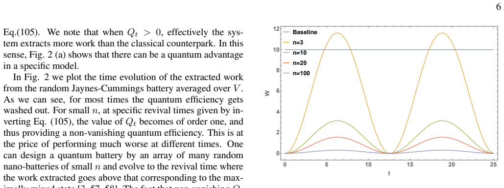
Starting from the closed-system work definition $W(t)=\mathrm{Tr}[(\rho-\rho_t)H_0]$, the paper computes averages over unitary rotations $G$ of the interaction $V_G(t)=G^\dagger V(t)G$, and separately over random initial states and random measuring Hamiltonians. The central result is the exact average $\langle W\rangle_V=(E_0-\mathrm{Tr}H_0/n)[n/(n+1)+Q_t/(n^2-1)]$, with $Q_t=-2\sum_{j\neq k}\cos(\theta_j-\theta_k)$ for eigenvalues $e^{i\theta_j}$ of $K=\mathcal{T}\exp(-i\int_0^t V(s)\,ds)$; for large $n$ this becomes $(E_0-\mathrm{Tr}H_0/n)(1+Q_t/n^2)$. The fluctuations obey an upper bound of the form $C' M(n) n^{-2}$, where $M(n)$ is a sum of phase factors of $K$; when the phases are generic, as in the circular unitary ensemble, $M(n)$ concentrates near zero, giving the claimed $n^{-2}$ decay. The paper applies this machinery to the Jaynes-Cummings model, finding revival times at which $Q_t$ becomes of order one and the battery beats the infinite-temperature baseline, and to adiabatic random batteries, whose fluctuations scale as $E_0^2/n^2$ for large $n$.
Load-bearing premise
The proof of fluctuation concentration relies on all initial-state occupation probabilities being uniformly small, no larger than a constant divided by the Hilbert-space dimension; for pure or highly occupied initial states, the claimed $n^{-2}$ decay of fluctuations is not established.
Editorial extensions
If this is right
- If the typicality result holds, an experimentalist can engineer a battery by fixing the spectrum of the driving operator and then ignore almost all other details of the drive in the large-$n$ limit.
- At revival times where $Q_t$ is of order one, an array of small random batteries can extract more work than the infinite-temperature classical baseline, at the price of performing worse at other times.
- For generic random spectra the quantum efficiency factor $Q_t/n^2$ decays, so large random batteries behave essentially like devices that drive the system toward the maximally mixed state, but using limited energetic resources.
- Adiabatic random batteries also concentrate, with fluctuations scaling as $E_0^2/n^2$; for non-degenerate Hamiltonians the quantum amplification is washed out.
- The method yields a perturbation-theory route, via the Dyson series, so it applies to non-solvable models and to harmonic perturbations whose average work has a single maximum at predictable times.
Reading between the lines
- The revival-time amplification suggests a design principle: choose the spectrum of $K$ so its eigenvalues cluster near resonances, making $Q_t$ large over sustained intervals rather than spikes; the paper leaves the search for such models open.
- Because the work formulas are expressed through out-of-time-ordered correlators, the same concentration results could be used as a signature of scrambling or quantum chaos in driven systems, a connection the paper points to but does not develop.
- One testable extension is to replace full Haar rotations by local Haar averaging, which would show whether typicality survives spatial locality; the paper lists this as a direction for future work.
- The bounded-occupancy condition for concentration suggests that mixed initial states are where $n^{-2}$ fluctuations are guaranteed, while pure-state batteries may require different bounds or exhibit larger fluctuations; checking this numerically would clarify the theorem's reach.
Signed reviews
Editorial analysis
A structured set of objections, weighed in public.
Referee Report
Summary. The paper introduces a Haar-random ensemble of quantum batteries in which the initial state, the energy-measuring Hamiltonian, or the time-dependent driving are rotated by independent Haar unitaries with fixed spectra. The main result is an exact expression for the average extracted work, Eq. (12): <W>_V = (E0 - Tr H0 / n)(n/(n+1) + Q_t/(n^2-1)), with Q_t a spectral form factor of the interaction-picture evolution operator. The paper claims that this average is typical, with fluctuations of order n^-2, via the bound in Eq. (18) and the S4-irrep calculation in Appendix VII. It then applies the formalism to the Jaynes-Cummings model, to second-order Dyson perturbation theory for harmonic drives, and to adiabatic quantum batteries, where a second typicality result is claimed in Eqs. (28)-(29).
Significance. If the central claims hold, the paper gives a clean, parameter-free way to compute average work in random batteries and identifies the spectral factor that can produce quantum advantage at revivals. The Haar-averaging derivation of Eq. (12) is transparent and appears correct, and the applications to exactly solvable and perturbative models are potentially useful. The advertised typicality results, however, are not established: the fluctuation bound relies on an invalid inequality, and the adiabatic asymptotic formula is inconsistent with the preceding exact formula. Since these are the two headline claims, the present version is not publishable without substantial revision.
major comments (2)
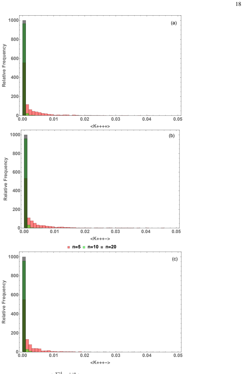
- [Sec. III, Eq. (18); App. VII B] The inequality in Eq. (18), |Tr[Pi_i (rho tensor H0)^{tensor 2}]| <= (Tr H0)^2, is false for indefinite H0. Positivity of Pi_i does not imply |Tr(Pi_i B)| <= |Tr B| unless B is positive semidefinite, and (rho tensor H0)^{tensor 2} is not PSD when H0 has negative eigenvalues. A concrete counterexample is n=2, rho=|1><1|, H0=diag(1,-1): the right-hand side is (Tr H0)^2=0, while Tr[Pi_sym (rho tensor H0)^{tensor 2}] = 1. This bound is the step that converts the traces over S4 irreps into Delta W^2_V <= C' M(n) n^{-2}; therefore the typicality theorem for general initial states is unproved. The appendix implicitly concedes this in VII B ('We see from the bound above that this is not enough to prove concentration'), and the alternative proof there requires p_i <= gamma/n, which excludes the pure and highly occupied initial states that the paper elsewhere keeps in scope. The numerical CUE analysis of M(n) in Fig. 4 concerns only the spectral factor and does not repair the invalid state-dependent inequality.
- [Sec. IV C, App. VII F, Eqs. (28)-(29)] The reduction of Eq. (28) to Eq. (29) is not correct. For non-degenerate d_i=1, the term retained in Eq. (29) equals Sum_{i,j} p_i^2 eps_j^2/(n^2-1), i.e., (Sum_i p_i^2)(Sum_j eps_j^2)/(n^2-1), not Tr(rho0 H0)^2/n^2 = E0^2/n^2. For a pure initial state this retained term is O(Tr H0^2/n^2) and can be O(1) when Tr H0^2 is extensive, while Eq. (29) predicts O(eps_i0^2/n^2). The dropped terms also scale as Tr H0^2/n^3, which is the same order as the claimed result when Tr H0^2 ~ n. Concretely, for n=2, rho0=|1><1| and H0=diag(1,-1), Eq. (28) gives Delta W^2_ad = 1/3, whereas Eq. (29) gives 1/4. The adiabatic typicality claim therefore does not follow from the calculation presented.
minor comments (6)
- [Throughout] There are several typos, including 'Hamitonian' in Sec. I, 'counterpark' in Sec. IV A, and 'attenued' in Sec. III; please proofread the manuscript.
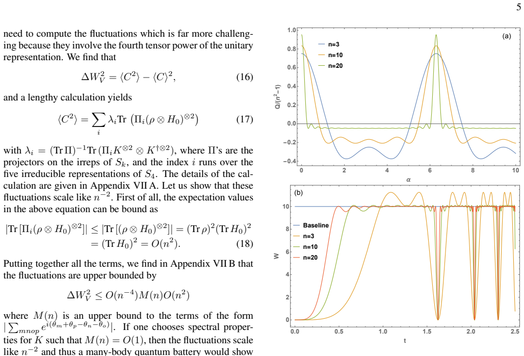
- [Sec. IV A and Fig. 2] The caption lists n=3 while the text says n=2 and the legend shows n=3,10,20; please harmonize the dimension labels.
- [App. VII A, after Eq. (54)] The projector trace expression 'Tr (Pi(st)' is missing a closing parenthesis and is not readable; please re-typeset the equation.
- [Sec. IV C] The definition of D_alpha should read (tr Pi^1_alpha, ..., tr Pi^R_alpha); the trace is missing in the displayed formula.
- [App. VII B, Eq. (87)] The same invalid inequality from Eq. (18) is restated as 'true because the projector operators are positive'; this should be removed or corrected.
- [Eq. (13) and Fig. 2(a)] The sign convention between Q_t = -2 Sum cos in Eq. (13) and the positive values labeled Q/(n^2-1) in Fig. 2(a) should be clarified; if the plotted quantity is the cosine sum without the minus sign, define it as such.
Circularity Check
No circular reduction: the main work formula is Haar-derived with Q_t defined from the spectrum, and the self-citations used are independent technical results; the proof gap in Eq. (18) is a correctness issue, not a circularity.
full rationale
The paper's central formulas are derived by first-principles Haar averaging, not by fitting or by defining the output in terms of the input. The average work in Eq. (12) is a nontrivial trace calculation in which Q_t is fixed as Q_t = -2 sum_{j != k} cos(theta_j - theta_k) from the eigenvalues of K, and the same Q_t then determines the work; there is no parameter tuned to reproduce any measured work value. The fluctuation calculation is likewise an explicit S4-projector computation rather than an assumed concentration result. The self-citations in the paper are limited to standard Haar-averaging techniques ([41,42], Hamma et al.) and the adiabatic connectibility criterion [62] (Hamma and Zanardi); these are parameter-free published mathematical tools whose assumptions do not include the target typicality statement, so they are real evidence rather than load-bearing self-citation. The numerical CUE analysis of Q and M(n) is used as evidence about spectral statistics, not as a fitted input. The appendix does contain an explicit limitation: the general p_i <= 1 bound is said to be 'not enough to prove concentration,' and the inequality in Eq. (18), |Tr[Pi_i(rho otimes H0)^{otimes 2}]| <= |Tr[(rho otimes H0)^{otimes 2}]| = (Tr H0)^2, is not valid for non-positive H0; however, an invalid bound or an unproved concentration claim is a proof/correctness gap, not a circular reduction of the advertised result to its inputs. No step in the derivation chain equates a prediction with an input by construction, so there is no significant circularity.
Assumptions & free parameters
assumptions (6)
- domain assumption The battery is a closed quantum system evolving unitarily, and work is Tr[(rho - rho_t) H0].
- domain assumption Noise is modeled by Haar-random unitaries G that rotate the perturbation, the initial state, or the Hamiltonian while preserving their spectra.
- standard math Standard Haar integration formulas and Schur-Weyl projectors for S2 and S4 are used to compute averages.
- ad hoc to paper For the fluctuation concentration, the initial state must have occupation probabilities p_i bounded by gamma/n, or one must use the (invalid or insufficient) bounds in Appendix VII B.
- ad hoc to paper Typical spectra from the Circulant Unitary Ensemble have M(n) = O(1), where M(n) bounds sums of phase exponentials.
- domain assumption Adiabatic evolution conserves populations in the spectral subspaces, and H0 and H1 are iso-degenerate connectible.
Cite this review
Pith. "Pith review of Random Quantum Batteries." pith.science (2026). https://pith.science/paper/GWALNXWY
@misc{pith2026190808064,
  author       = {Pith},
  title        = {Pith review of: Random Quantum Batteries},
  year         = {2026},
  howpublished = {\url{https://pith.science/paper/GWALNXWY}},
  note         = {Machine review of arXiv:1908.08064}
}
read the original abstract
Quantum nano-devices are fundamental systems in quantum thermodynamics that have been the subject of profound interest in recent years. Among these, quantum batteries play a very important role. In this paper we lay down a theory of random quantum batteries and provide a systematic way of computing the average work and work fluctuations in such devices by investigating their typical behavior. We show that the performance of random quantum batteries exhibits typicality and depends only on the spectral properties of the time evolving operator, the initial state and the measuring Hamiltonian. At given revival times a random quantum battery features a quantum advantage over classical random batteries. Our method is particularly apt to be used both for exactly solvable models like the Jaynes-Cummings model or in perturbation theory, e.g., systems subject to harmonic perturbations. We also study the setting of quantum adiabatic random batteries.
Figures
Figures from the paper (1 more)
Reference graph
Works this paper leans on
-
[1]
That is, averaging over the spectra does not give any amplificationQt
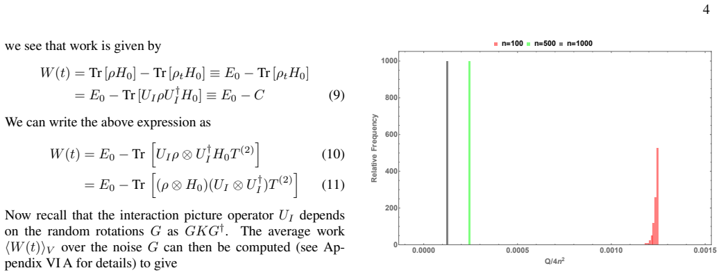
We see that for large n the peak of the distribution moves towards zero. That is, averaging over the spectra does not give any amplificationQt. How typical is the behavior of a random quantum battery in the largen limit? If there is typicality, an optimal strategy for random quantum batteries would consist in fixing the optimal spectrum ofK and then knowing...
-
[2]
We now have Πi αΠj β =δij ifα =β, but otherwise they are not necessarily orthogonal
(22) because the populations in thei−th subspace are conserved by the adiabatic evolution. We now have Πi αΠj β =δij ifα =β, but otherwise they are not necessarily orthogonal. We see that the work depends on the choice ofU as WU = ∑ ij piϵj 0 ( Tr(Πi 0Πj 0)− Tr(Πi 0Πj 1) ) = ∑ ij piϵj 0 ( diδij− Tr(Πi 0UΠj 0U†) ) (23) We can now perform the average over t...
-
[3]
F. Campaioli, F.A. Pollock, S. Vinjanampathy, Quantum Batter- ies. In: Binder F., Correa L., Gogolin C., Anders J., Adesso G. (eds) Thermodynamics in the Quantum Regime. Fundamental Theories of Physics, vol 195. Springer, Cham (2018)
work page 2018
- [4]
-
[5]
D. Ferraro, M. Campisi, G. Andolina, V . Pellegrini, M. Polini, Phys. Rev. Lett 120(11), 117702 (2018)
work page 2018
-
[6]
G. M. Andolina, D. Farina, A. Mari, V . Pellegrini, V . Giovan- netti, M. Polini. Phys. Rev. B, 98:205423 (2018)
work page 2018
-
[7]
G. M. Andolina, M. Keck, Andrea Mari, M. Campisi, V . Gio- vannetti, M. Polini. Phys. Rev. Lett., 122:047702 (2019)
work page 2019
-
[8]
G. M. Andolina, M. Keck, A. Mari, V . Giovannetti, M. Polini. Phys. Rev. B, 99:205437 (2019)
work page 2019
Show all 75 references
-
[10]
T. P. Le, J. Levinsen, K. Modi, M. Parish, F. A. Pollock. ArXiv e-prints (2017)
2017
-
[11]
L. A. Correa, J. P. Palao, G. Adesso, D. Alonso. Phys. Rev. E, 87:042131 (2013)
2013
-
[12]
Watanabe, B
G. Watanabe, B. P. Venkatesh, P. Talkner, A. del Campo.Phys. Rev. Lett., 118:050601 (2017)
2017
-
[13]
A. Levy, R. Alicki, R. Kosloff, Phys. Rev. E 85, 061126 (2012)
2012
-
[14]
J. ˚Aberg. Nat. Comm., 4:1925 (2013)
2013
-
[15]
A. M. Alhambra, L. Masanes, J. Oppenheim, C. Perry. Phys. Rev. X, 6:041017 (2016)
2016
-
[16]
A. M. Alhambra, G. Styliaris, N. A. Rodriguez-Briones, J. Sikora, E. Martin-Martinez. arXiv e-prints, arXiv:1902.02357 (2019)
2019 arXiv
-
[17]
Alicki and D
R. Alicki and D. Gelbwaser-Klimovsky. New J. of Phy. , 17(11):115012 (2015)
2015
-
[18]
Masanes, J
L. Masanes, J. Oppenheim, Nat. Comm., 8:14538 (2017)
2017
-
[19]
Alicki, J
R. Alicki, J. Phys. A 12, L103 (1979); R. Kosloff, J. Chem. Phys. 80, 1625 (1984)
1979
-
[20]
Popescu, A
S. Popescu, A. J. Short , A. Winter . Nature Physics 2, pp 754- 758 (2006)
2006
-
[21]
Skrzypczyk, A
P. Skrzypczyk, A. J. Short, S. Popescu. Nat. Comm., 5:4185 (2014)
2014
-
[22]
Kasprzak et al., Nature Mat
J. Kasprzak et al., Nature Mat. 9, pp 304-308(2010)
2010
-
[23]
Niemczyk et al, Nature Physics 6, 772 - 776 (2010)
T. Niemczyk et al, Nature Physics 6, 772 - 776 (2010)
2010
-
[24]
Linden, S
N. Linden, S. Popescu, P. Skrzypczyk. Phys. Rev. Lett. , 105:130401 (2010)
2010
-
[25]
Anders, M
J. Anders, M. Esposito, New J. of Phy., 19(1):010201 (2017)
2017
-
[26]
Sparaciari, J
C. Sparaciari, J. Oppenheim, T. Fritz, Phys. Rev. A 96, 052112 (2017), 1607.01302
2017 arXiv
-
[27]
Nath Bera, A
M. Nath Bera, A. Riera, M. Lewenstein, Z. B. Khanian, and A. Winter, Quantum 3, 121 (2019)
2019
-
[28]
F. G. S. L. Brand ˜ao, M. Horodecki, J. Oppenheim, Joseph M. Renes, R. W. Spekkens. Resource theory of quantum states out of thermal equilibrium. Phys. Rev. Lett., 111:250404 (2013)
2013
-
[29]
Demkowicz-Dobrza ´nski, J
R. Demkowicz-Dobrza ´nski, J. Kołody´nski, and M. Gut ¸˘a. Nat. Comm., 3:1063 (2012)
2012
-
[30]
M. F. Frenzel, D. Jennings, and T. Rudolph. Phys. Rev. E , 90(5):052136 (2014)
2014
-
[31]
Friis, M
N. Friis, M. Huber. Quantum, 2:61 (2018)
2018
-
[32]
Roberts, B
D.A. Roberts, B. Yoshida, B. J. High Energ. Phys. (2017) 2017: 121
2017
-
[33]
Gallego, J
R. Gallego, J. Eisert, H. Wilming. N. J. of Phys., 18(10):103017 (2016)
2016
-
[34]
B. Yan, L. Cincio, W. H. Zurek, arXiv:1903.0265
1903
-
[35]
Goold, M
J. Goold, M. Huber, A. Riera, L. del Rio, P. Skrzypczyk. J. of Phys. A: Math. and Th., 49(14):143001 (2016)
2016
- [36]
-
[37]
Rossini, G.-M
D. Rossini, G.-M. Andolina, M. Polini, Phys. Rev. B 100, 115142 (2019)
2019
-
[38]
Chenu, J
A. Chenu, J. Molina-Vilaplana, A. del Campo, Quantum 3, 127 (2019)
2019
-
[39]
Chenu, I
A. Chenu, I. L. Egusquiza, J. Molina-Vilaplana, A. del Campo, Sci. Rep. 8, 12634 (2018)
2018
-
[40]
J. G. Richens, L. Masanes Nat. Comm. 7,13511 (2016)
2016
-
[41]
Allahverdyan, R
A.E. Allahverdyan, R. Balian, T.M. Nieuwenhuizen, Europhys. Lett. 67, 565 (2004)
2004
-
[42]
Zyczkowski, P
K. Zyczkowski, P. Horodecki, A. Sanpera, M. Lewenstein, Phys. Rev. A 58 (1998) 883
1998
-
[43]
Hamma, S
A. Hamma, S. Santra, P. Zanardi, Phys. Rev. Lett. 109, 040502 (2012)
2012
-
[44]
Hamma, S
A. Hamma, S. Santra, P. Zanardi, Phys. Rev. A 86, 052324 (2012)
2012
-
[45]
Alicki, R
R. Alicki, R. Horodecki, P. Horodecki, R. Horodecki, Open Syst. Inform. Dynam. 11, 205 (2004)
2004
-
[46]
˚Aberg, Phys
J. ˚Aberg, Phys. Rev. Lett., 113:150402 (2014)
2014
-
[47]
Brandner, M
K. Brandner, M. Bauer, M.T. Schmid, U Seifert, New J. of Phy., 17(6):065006 (2015)
2015
-
[48]
Francica, J
G. Francica, J. Goold, F. Plastina, Phys. Rev. E , 99:042105 (2019)
2019
-
[49]
Korzekwa, M
K. Korzekwa, M. Lostaglio, J. Oppenheim, D. Jennings, New J. of Phy., 18(2):023045 (2016)
2016
-
[50]
C. L. Latune, I. Sinayskiy, F. Petruccione, Sci. Rep., 9:3191 (2019)
2019
-
[51]
Lostaglio, K
M. Lostaglio, K. Korzekwa, D. Jennings, T. Rudolph, Phys. Rev. X, 5:021001 (2015) 9
2015
-
[52]
Marvian, R
I. Marvian, R. W. Spekkens, P. Zanardi, Phys. Rev. A , 93:052331 (2016)
2016
-
[53]
Streltsov, G
A. Streltsov, G. Adesso, M. B. Plenio, Rev. of Mod. Phys. , 89(4):041003 (2017)
2017
-
[54]
Juli ´a-Farr`e, T
S. Juli ´a-Farr`e, T. Salamon, A. Riera, M. N. Bera, M. Lewen- stein, arXiv:1811.04005v2
-
[55]
J. G. Richens, L. Masanes, Nat. Comm., 7:13511 (2016)
2016
- [56]
-
[57]
Campos Venuti, N
L. Campos Venuti, N. T. Jacobson, S. Santra, P. Zanardi, Phys. Rev. Lett. 107, 010403 (2011)
2011
-
[58]
Jaynes, F.W
E.T. Jaynes, F.W. Cummings, Proc. IEEE. 51 (1): 89-109 (1963)
1963
-
[59]
F. C. Binder, S. Vinjanampathy2, K. Modi, J. Goold, New J. Phys. 17 075015 (2015)
2015
-
[60]
Campaioli, F
F. Campaioli, F. A. Pollock, F. C. Binder, L/ C´eleri, J. Goold, S. Vinjanampathy, K. Modi, Phys. Rev. Lett., 118:150601 (2017)
2017
-
[61]
Farhi, J
E. Farhi, J. Goldstone, S. Gutmann, J. Lapan, A. Lundgren, D. Preda, Science 292, 472 (2001); T. Albash,D. A. Lidar, Rev. Mod. Phys. 90, 015002 (2018)
2001
-
[62]
Quiroz, Phys
G. Quiroz, Phys. Rev. A 99, 062306 (2019)
2019
-
[63]
del Campo, J
A. del Campo, J. Goold, M. Paternostro. Sci. Rep., 4 (2014)
2014
-
[64]
Hamma, P
A. Hamma, P. Zanardi, Phys. Rev. A 69, 062319 (2004)
2004
-
[65]
A. C. Santos, B. akmak, S. Campbell, N. T. Zinner, Phys. Rev. E 100, 032107 (2019)
2019
-
[66]
Wang, T.-S
S.-D. Wang, T.-S. Kuo, C.-F. Hsu,IEEE Trans.Autom. Con- trol, vol. AC-31, no. 7, pp. 654-656 (1986); J. M. Saniuk, I. B. Rhodes, IEEE Trans. Autom. Control 32(8), pp. 739-740 (1987); T. Mori,IEEE Trans.Autom. Control, 33(11), p. 1088 (1988)
1986
-
[67]
Funo, J.-N
K. Funo, J.-N. Zhang, C. Chatou, K. Kim, M. Ueda, A. del Campo, Phys. Rev. Lett., 118:100602 (2017)
2017
-
[68]
Styliaris, L
G. Styliaris, L. Campos Venuti, P. Zanardi, Phys. Rev. A 97, 032304 (2018)
2018
-
[69]
Rezakhani, W.-J
A.T. Rezakhani, W.-J. Kuo, A. Hamma, D.A. Lidar, P. Zanardi, Phys. Rev. Lett. 103, 080502 (2009)
2009
-
[70]
Mirsky, Mon
L. Mirsky, Mon. Math., 79 (4) (1975); Also, see the notes on spectral methods available at https://www.overleaf.com/read/wdxknyfmdnww. 10 VI. APPENDIX A. Calculation of ∆W 2 ρ SinceW = 0 andW 2 = TrW· TrW = Tr(W⊗W ), we see that ∆W 2 =⟨W 2⟩ =⟨Tr(ρδH0)⊗2⟩ = Tr [ ⟨ρ⊗2⟩δH⊗2] . Th...
1975
-
[71]
Note that Tr(U2U†
+ Tr(U2U† 2) 2 λ− = Tr((U2⊗U† 2)Π−) Tr(Π−) = 2 n(n− 1) Tr(U2)Tr(U† 2)− Tr(U2U† 2) 2 . Note that Tr(U2U†
-
[72]
We can use at this point the eqns
= Tr(U† 2U2) = n +O(t3). We can use at this point the eqns. (40) again. After a rapid calculation we see that (up to corrections of ordert3), we have λ± = n2±n−nTr(A2)− Tr(A)2 n2±n (116) and thus λ+ +λ− 2 = n2− 1 + Tr(A)2−nTr(A2) n2− 1 λ+−λ− 2 =−Tr(A)2−nTr(A2) n(n2−n) (117) 22...
-
[73]
At timet = 0, the system is described by the eigenvalue equation ˆH0ψm =Emψm, (121) and thus the wavefunction as a function of time can be written as ψ(t) = ∑ m cme−iEmtψm
Example: Harmonic perturbations Let us now consider the example of an-level system. At timet = 0, the system is described by the eigenvalue equation ˆH0ψm =Emψm, (121) and thus the wavefunction as a function of time can be written as ψ(t) = ∑ m cme−iEmtψm. (122) We consider no...
-
[74]
It can be shown that the evolution of the projector operators can be written as Πi α(t) =UtΠi α(0)U† t. (139) Thus, the time evolution of the Hamiltonian for an adiabatic system can be written as H(t) = R∑ i=1 ϵi(t)UtΠi 0U† t, (140) where the while the density matrix asρ(t) =∑...
-
[75]
(141) We now haveΠi αΠj β =δij ifα =β, but otherwise they are not necessarily orthogonal. Let us write the work as W = ∑ i,j piϵj 0 ( Tr(Πi 0Πj 0)− Tr(Πi 0Πj 1) ) = ∑ i,j piϵj 0 ( diδij− Tr(Πi 0GΠj 0G†) ) (142) We can now perform the average over the unitary transformationU. W...
-
[76]
We thus find that the maximum gain that one can has from degeneracy is ⟨W⟩ad−⟨W⟩≤ Tr(ρH0) ∑ id2 i−n n , (155) from which we obtain ⟨W⟩ad≤E0(1 +c)− Tr(H0) n (156) withc = ∑ id2 i−n n
Thus the spectral norm isσmax(B) = max(0, 1 n ∑ ipiϵi 0). We thus find that the maximum gain that one can has from degeneracy is ⟨W⟩ad−⟨W⟩≤ Tr(ρH0) ∑ id2 i−n n , (155) from which we obtain ⟨W⟩ad≤E0(1 +c)− Tr(H0) n (156) withc = ∑ id2 i−n n
Reviewed August 14, 2026 · model on record in the stance chip above.
Discussion (0). Continue with ORCID to comment.