REVIEW 3 major objections 4 minor 1 cited by
The paper establishes that geometrically local open lattice models with stationary Gaussian environments can be digitally simulated with near-optimal resources: O(Nt(Nt/δ)^{o(1)}) gates and depth O(t(Nt/δ)^{o(1)}), with depth independent of
Reviewed by Pith at T0; open to challenge. T0 means a machine referee read the full paper against a public rubric. the ladder, T0–T4 →
Near-optimal quantum simulation algorithms for non-Markovian and Markovian open lattice models, including local-observable circuits with size-independent depth.
T0 review reviewed 2026-08-05 challenge →
load-bearing objection Strong algorithmic results for non-Markovian lattice simulation, but the central resource count has an arithmetic slip that needs fixing, and some key local-error support is unpublished. the 3 major comments →
Optimizing digital quantum simulation of open quantum lattice models
The pith
A machine-rendered reading of the paper's core claim, the machinery that carries it, and where it could break.
The reading
Core claim
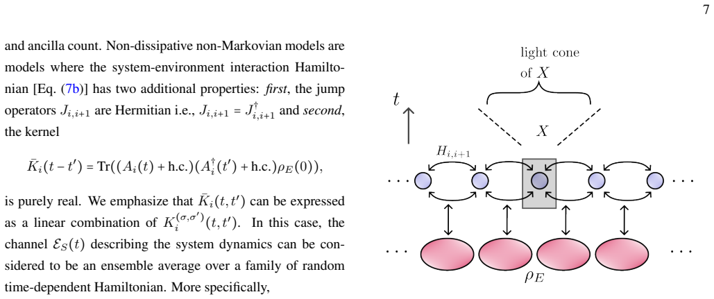
Theorem 1 is the load-bearing statement. Under assumption Eq. (15), the channel E_S(t) generated by a geometrically local Hamiltonian with nearest-neighbour system-bath couplings to a stationary Gaussian environment can be approximated within trace distance δ by a digital circuit using O(Nt(Nt/δ)^{1/p}) geometrically local gates and Õ(N(Nt/δ)^{1/(p+1)}) ancillas for every p>0; choosing p to grow slowly yields O(Nt(Nt/δ)^{o(1)}) gates. The proof decomposes the total Hamiltonian into odd/even bond groups, applies a P-th order Trotter formula in the interaction picture, and bounds the error despite the unbounded bath operators by using Gaussian Wick contractions, giving Lemma 1 with error O((P
What carries the argument
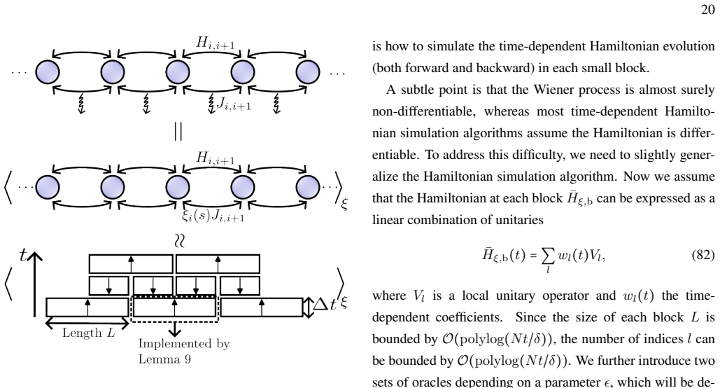
The central mechanism is a Trotterization lemma for open systems (Lemma 1), which treats the full system-environment Hamiltonian as a lattice Hamiltonian with odd/even bond decomposition and shows that a P-th order Trotter formula approximates the system channel with error O((P s_P)^P N t (t/T)^P), despite the bath being unbounded. The companion machinery is a three-step environment reduction: discretize the continuum of bath modes into polynomial segments in time, Trotterize, then truncate each bosonic mode to a qudit; Gaussian Wick contractions convert unbounded bath operators into bounded kernel integrals. For local observables, Lieb-Robinson light cones for open systems make the Trotter
Load-bearing premise
Each bond must have its own independent Gaussian environment, and in the general dissipative case the coupling functions must be smooth and decay faster than any polynomial; neither a shared or spatially correlated bath nor an algebraic-decay coupling is covered.
What would settle it
The most direct check is a two-site chain with coupling v(t)=e^{-t^2} (both smooth and superpolynomially decaying, satisfying Eq. (15)): compute the exact channel by numerical integration of the full system-bath model, run the paper's discretize-Trotterize-quditize circuit at a fixed p, and compare trace distances. If the number of gates needed per unit error exceeds O(Nt(Nt/δ)^{1/p}) by a non-subpolynomial factor, Theorem 1 needs revision. A second probe is to allow a single shared Gaussian bath between the two bonds, K_{1,2}(τ)≠0, which violates the per-bond independence assumption Eq. (8) a
If this is right
- Even with memory, simulation cost matches closed-system near-optimal scaling: O(Nt(Nt/δ)^{o(1)}) gates, so the only penalty is subpolynomial.
- Parallelized depth stays O(t(Nt/δ)^{o(1)}), close to the linear-time lower bound.
- For D-dimensional lattices, local-observable simulation needs depth O(t(t^{D+1}/δ)^{1/p}) independent of N, making pre-fault-tolerant implementations more plausible.
- Non-dissipative non-Markovian models need no ancillas and no smoothness beyond bounded L1 kernels, since their dynamics is an ensemble of random local Hamiltonians.
- Markovian Lindbladians with commuting jump operators can be simulated with O(Nt polylog(Nt/δ)) gates for Hermitian jumps with Q-RAM, or O(Nt(Nt/δ)^{1/3}) gates for non-Hermitian jumps via local dilation.
Where Pith is reading between the lines
- The per-bond independence assumption (Eq. 8) is likely the main boundary: spatially correlated Gaussian baths, common for phonons, are not covered, and closing that gap would require a non-scalar Wick-contraction analysis.
- The paper's discussion implies an essentially exact equivalence, up to N^{o(1)} overhead, between continuous-time and discrete-time definitions of open-system phases.
- A natural next test is whether the smooth-superpolynomial assumption (Eq. 15) can be weakened to algebraic decay with bounded derivatives, since the non-dissipative theorem already removes smoothness; a positive answer would extend the result to more realistic spectral densities.
- The ancilla count Õ(N(Nt/δ)^{1/(p+1)}) sits above the naive O(N) lower bound suggested by channel rank; tightening either side would determine whether ancilla recycling is fundamentally limited or merely an artifact of the construction.
Editorial analysis
A structured set of objections, weighed in public.
Referee Report
Summary. The paper develops digital quantum simulation algorithms for geometrically local open lattice models coupled to stationary Gaussian environments. It presents a non-Markovian algorithm based on temporal discretization of the environment, higher-order Trotterization, and qudit truncation, claiming near-optimal gate counts O(N t (N t/δ)^{1/p}) and ancilla counts Õ(N (N t/δ)^{1/(p+1)}) (Theorem 1), with an N-independent circuit depth for local observables (Theorem 3). For non-dissipative models it gives ensemble-based algorithms with no ancillas (Theorems 2 and 4). For Markovian models with commuting jump operators it proposes a Wiener-process sampling algorithm with Q-RAM (Theorem 5) and a locally dilated Hamiltonian achieving third-order error scaling (Theorem 6). Proofs are outlined in the main text and detailed in an extensive supplemental material.
Significance. If the results hold, the non-Markovian theorems close most of the asymptotic gap between simulating closed and open lattice models for Gaussian environments, and the Markovian results improve the N-scaling for commuting jump operators. The paper's strengths are its explicit, non-asymptotic resource bounds, the absence of fitted parameters, the careful Wick-contraction-based Trotter analysis, and the candid acknowledgment of the main limitations (per-bond independent environments, Eq. (8), and the smoothness/decay assumption Eq. (15)). The central non-Markovian claim is a provable upper bound rather than a numerical heuristic. However, the proof of the main theorem contains an internal arithmetic inconsistency in the resource count, and the Markovian dilation claim is only leading-order in the time step, so the headline claims are not fully justified as written.
major comments (3)
- [Section III.B.5, Eq. (54)] The displayed norm bound O(r√d/η) does not follow from the preceding factors. With 2j_max(2r/η+2) active modes, |C^n_{i,j}(t)|≤C0√η, and ‖P_d b^n_{i,j}P_d‖≤√d, the product is O(j_max r√d/√η), not O(r√d/η). This distinction is load-bearing: using the printed O(r√d/η) in Eq. (55) gives a circuit-depth exponent 1/(2p)+1/(p+1), which exceeds 1/p for p>1 and breaks Theorem 1's claimed O(Nt(Nt/δ)^{1/p}) scaling. The derivation supports the stronger bound, so the theorem may be recoverable, but the text as written is internally inconsistent and must be corrected.
- [Section II.B.3 and III.F, Theorem 6] Theorem 6 and the subsequent complexity claim O(Nt(Nt/δ)^{1/3}) depend on the per-step dilation error Rdia=O(Δt^4). The proof controls only the leading-order coefficient G^(4)_dia; the text explicitly states that all-order remainder analysis is left open. Since the total simulation error is T times the per-step remainder, an uncontrolled remainder growing with N or with inverse powers of Δt would invalidate the stated T=Θ(t(Nt/δ)^{1/3}) and the associated gate count. This is a fundamental gap in the Markovian claim, not a presentation issue; the theorem statement should either include a full remainder bound or be qualified as a leading-order analysis.
- [Section III.D, Lemma 11 and Theorem 3] The N-independent local-observable depth claim relies on a Lieb-Robinson bound for open systems with memory imported from Ref. [64], an arXiv preprint by two of the same authors. This is a load-bearing external result. Please include a self-contained statement (and proof or precise citation to a refereed version) of the exact bound used, and verify that the hypotheses of Ref. [64] match the model here, in particular the bounded-memory-kernel condition and the treatment of the discretized environment in Theorem 3.
minor comments (4)
- [Theorem 2] The theorem states an ensemble whose expectation approximates E_S(t), but does not include the finite-sample error of the classical Gaussian sampling. Unlike Theorem 4, no 1/δ^2 sampling overhead is mentioned. Please state the number of samples and the total sampled gate count explicitly.
- [Abstract and Theorem 1] The abstract's O(Nt(Nt/δ)^{o(1)}) claim is obtained by letting p grow slowly with N,t,δ, while Theorem 1 states O(Nt(Nt/δ)^{1/p}) for any fixed p>0. The distinction between the two statements should be clarified in the main text, since a fixed p does not yield o(1).
- [Theorems 1–4] The main text says the results extend to higher-dimensional lattices, but Theorems 1 and 2 are stated for a one-dimensional lattice. Please state the dimension explicitly or add a sentence explaining how the D-dimensional generalization follows.
- [Section III.E.2] The 'quantum Ito solver oracle' O_qito is an invented resource, and the resulting statement is conditional on its existence. This is presented clearly in the text, but it should be explicitly marked as a conditional observation rather than a theorem or algorithmic contribution, so that readers do not mistake it for a concrete digital simulation method.
Circularity Check
No circularity: complexity bounds are derived from stated model assumptions; same-author citations are independent support.
full rationale
The paper's claims are resource upper bounds, not empirical predictions, and no parameter is fitted to the target quantity. Theorem 1 is obtained by composing explicit, state-dependent error bounds: Lemma 1 (Trotterization), Lemmas 2-4 (discretization), Lemmas 5-6 (quditization), with η and d chosen in Eqs. (48) and (51) to split the error into thirds. The gate/depth/ancilla counts in Sec. III.B.5 are direct arithmetic consequences of those choices. The inputs (stationarity, Gaussianity, per-bond factorization Eq. (8), smooth superpolynomial decay Eq. (15)) are assumptions, not the output complexity, so there is no self-definitional reduction. The same holds for Theorems 2, 5 and 6. The only overlapping-author citations are Ref. [64] (LR bound for open systems with memory, R. Trivedi) and Ref. [81] (closed-system local Trotter error, Trivedi & Cirac, manuscript in preparation); they are load-bearing for the local-observable Theorems 3-4 and noise-robustness discussion, but they are cited as independent parameter-free theorems that do not assume the present result, and the paper supplies its own extension argument in Lemma 7 and Supplement V.A. The paper itself flags open limitations (leading-order-only dilation analysis after Theorem 6; open problem of arbitrary-order local dilation), which are not circularity. The arithmetic concern about Eq. (54) vs Eq. (55) (O(r√d/η) vs O(r√d/√η)) is a correctness risk in the printed proof, not a circular reduction: even if the stated norm bound is inaccurate, the theorem is not forced by its own inputs by definition.
Axiom & Free-Parameter Ledger
axioms (6)
- domain assumption Environment is stationary and Gaussian; correlators satisfy Wick's theorem and time-translation invariance.
- domain assumption Initial system-environment state is a product state; main text takes vacuum bath, supplement extends to general Gaussian states.
- domain assumption Memory kernels and coupling functions satisfy smoothness and decay conditions Eq. (13)/(15): uniformly bounded L-infinity and L1 norms, bounded derivatives, superpolynomial decay.
- domain assumption Environments attached to different bonds are independent: K_{i,j}=K_i δ_{i,j} (Eq. 8), and system-environment couplings are nearest-neighbor.
- domain assumption Jump operators commute for the Markovian results: [J_{i,i+1}, J_{j,j+1}]=[J_{i,i+1}, J_{j,j+1}^†]=0 for i≠j.
- standard math External bounds from cited literature are valid: kernel-sensitivity bound (Lemma 3 from Ref. [65]), Lieb-Robinson bound for open systems with memory (Ref. [64]), Hamiltonian simulation with linear combinations of unitaries (Ref. [69]), and local-error analysis assumptions (Ref. [81]).
invented entities (1)
-
Quantum Ito solver oracle O_qito
no independent evidence
Cite this review
Pith. "Pith review of Optimizing digital quantum simulation of open quantum lattice models." pith.science (2026). https://pith.science/paper/OXNTTU4I
@misc{pith2026250902268,
  author       = {Pith},
  title        = {Pith review of: Optimizing digital quantum simulation of open quantum lattice models},
  year         = {2026},
  howpublished = {\url{https://pith.science/paper/OXNTTU4I}},
  note         = {Machine review of arXiv:2509.02268}
}
read the original abstract
Many-body systems arising in condensed matter physics and quantum optics inevitably couple to the environment and need to be modelled as open quantum systems. While near-optimal algorithms have been developed for simulating many-body quantum dynamics, algorithms for their open system counterparts remain less well investigated. We address the problem of simulating geometrically local many-body open quantum systems interacting with a stationary Gaussian environment. Under a smoothness assumption on the system-environment interaction, we develop near-optimal algorithms that, for a model with $N$ spins and evolution time $t$, attain a simulation error $\delta$ in the system-state with $\mathcal{O}(Nt(Nt/\delta)^{o(1)})$ gates, $\mathcal{O}(t(Nt/\delta)^{o(1)})$ parallelized circuit depth and $\tilde{\mathcal{O}}(N(Nt/\delta)^{o(1)})$ ancillas. We additionally show that, if only simulating local observables is of interest, then the circuit depth of the digital algorithm can be chosen to be independent of the system size $N$. This provides theoretical evidence for the utility of these algorithms for simulating physically relevant models, where typically local observables are of interest, on pre-fault tolerant devices. Finally, for the limiting case of Markovian dynamics with commuting jump operators, we propose two algorithms based on sampling a Wiener process and on a locally dilated Hamiltonian construction, respectively. These algorithms reduce the asymptotic gate complexity on $N$ compared to currently available algorithms in terms of the required number of geometrically local gates.
Figures




Forward citations
Cited by 1 Pith paper
-
Dissipative preparation of injective tensor network states
Constructs geometrically local dissipative dynamics that prepare injective tensor network states in O(log(N/ε)) time for 1D MPS and high-injectivity higher-D cases.
Reference graph
Works this paper leans on
-
[1]
∣ρ⟫ denotes the vectorized density matrix of ρ on a doubled Hilbert space defined as ∑ i,j ρi,j ∣i⟩⟨ j∣ → ∑ i,j ρi,j ∣i⟩⊗∣j⟩∶= ∣ρ⟫. The trace norm on ∣ρ⟫ is defined as the trace norm of the original density matrix ρ as ∥∣ρ⟫∥tr = ∥ρ∥tr = Tr √ ρ†ρ. (S1)
-
[2]
Specfically, the vectorized Identity matrix is⟪I∣= ∑i⟨i∣⟨ i∣, with {⟨i∣} a set of orthonormal states
⟪O∣ denotes the vectorization of an observable O to a doubled Hilbert space as ∑ i,j Oi,j ∣i⟩⟨ j∣ → ∑ i,j ⟨i∣⊗⟨j∣ Oi,j =∶ ⟪O∣. Specfically, the vectorized Identity matrix is⟪I∣= ∑i⟨i∣⟨ i∣, with {⟨i∣} a set of orthonormal states
-
[3]
For simplicity, we still call the operator on the doubled Hilbert space as the superoperator
The superoperator on the original density matrix becomes an operator on the doubled Hilbert space. For simplicity, we still call the operator on the doubled Hilbert space as the superoperator
-
[4]
We will use the outline fonts to denote these superoperators, such as H, U, V, J, A⋯. Remark: In this Supplemental Material, if H is a Hamiltonian operator, the notation H corresponds to the commutator as H∣ρ⟫ = ∣[H, ρ]⟫. It U is a unitary operator, the notation U corresponds to the Adjoint as U∣ρ⟫= ∣U ρU†⟫
-
[5]
We use the symbol ⟨O⟩ to denote TrE(OρE(0)). Equivalently. in the doubled space notation, we use ⟨O⟩ to denote ⟪I∣EO∣ρE(0)⟫, with ⟪I∣E the vectorized Identity operator for the environmental space. 27
-
[6]
The diamond norm of a superoperator is defined as ∥O∥◇∶= max ∥∣ρ⟫∥tr=1,n ∥O⊗ In∣ρ⟫∥tr, (S2) where In denotes the Identity channel (in the doubled space) acting on an auxiliary system of dimension n, and ρ is any density matrix on the joint system composed of the supports of O and In
-
[7]
We introduce the adjoint expression for the superoperators as adO∶= [O,], AdV(⋅)∶= V(⋅)V†
-
[8]
Unless explicitly noted, a repeated Greek index, such as α, β, implies summation over that index. II. DETAILED PROOF OF LEMMA 1 A. Description of the Set up Suppose the original Hamiltonian is HSE(t)= N−1 ∑ i=1 Hi,i+1+ N−1 ∑ i=1 J † i,i+1Ai(t)+ Ji,i+1A† i(t), (S3) where Ji,i+1, Hi,i+1 act on the nearest neighbor sites i, i+ 1 with H† i,i+1 = Hi,i+1 and ∥H...
-
[45]
rewrite the remainder error expression Let us compute each term in the summand of Eq. (S19). For simplicity, we denote t2 = i∆t, t1 = (i− 1)∆t and ̃V(t1, 0) = ∏i−1 j=1 V(j∆t,(j− 1)∆t). Then, we are required to calculate ⟨USE(t, t2)[USE(t2, t1)− V(t2, t1)]̃V(t1, 0)⟩. (S25) From the explicit error remainder form in Ref. [18] and the procedure of transformin...
-
[46]
Counting the number of monomials Let’s fix k and w1⋯w2(k−1) at this moment. We start by bounding the number of nested commutators as well as the support of each monomial in J 1 P(τ). Then we can arrive at the bound of the number of monomials. In J 1 P(τ), there is at most (P + 1) bosonic operators Aα i which are multiplied together. Each time one of these...
-
[47]
(S2) for each monomial in the above counting
Bounding the diamond norm for each monomial Next, we need to bound the diamond norm defined in Eq. (S2) for each monomial in the above counting. As the monomial still involves the bosonic operator Aα i , we need to contract all of Aα i before bounding the superoperator norm. For a fixed Aα i Jα i,i+1, we now discuss all the possible ways it can contract w...
-
[48]
The Trotter error scaling Combining the above bounds on the number of monomials and on the superoperator norm of each monomial, we obtain ∥⟨USE(t, t1+ τ)V(t1+ τ, t1)× ∑ w1+⋯+w2(k−1)=P 1 ∏ l=k−1 AdVo,˜el−1(τ),˜el(τ)adw2l−1 Ho(˜el(τ))AdVe, ˜fl−1(τ), ˜fl(τ)adw2l He( ˜fl(τ))× (ckHo(˜ek−1(τ))+ dk−1He( ˜fk−1(τ)))̃V(t1, 0) P ! ∏ 2(k−1) i=1 wi! ⟩∥ ◇ ≤ ∑ w1+⋯+w2(k...
-
[49]
, (S163) almost surely in the simulation procedure. Equation (S163) thus allows us to discretize the integration ∫ s+∆s s W † sto(τ, 0)HSWsto(τ, 0)dτ into M pieces with M given below Eq. (S156) and α= 1/4. VII. DETAILED PROOF OF THEOREM 6 Here we consider an open quantum system of N sites. Its Markovian dynamics is described by dρS dt = L(ρS)=−i[HS, ρS]+ ...
-
[50]
A quantum algorithm to simulate Lindblad master equations
E. Borras and M. Marvian, A quantum algorithm to simulate lindblad master equations (2024), arXiv:2406.12748 [quant- ph]
work page internal anchor Pith review Pith/arXiv arXiv 2024
- [51]
-
[52]
A. Pereverzev and E. R. Bittner, The Jour- nal of Chemical Physics 125, 104906 (2006), https://pubs.aip.org/aip/jcp/article- pdf/doi/10.1063/1.2348869/15390215/104906_1_online.pdf
work page doi:10.1063/1.2348869/15390215/104906_1_online.pdf 2006
- [53]
-
[54]
A. Strathearn, P. Kirton, D. Kilda, J. Keeling, and B. W. Lovett, Nature communications 9, 3322 (2018)
work page 2018
- [55]
- [56]
-
[57]
D. Gribben, D. M. Rouse, J. Iles-Smith, A. Strathearn, H. Maguire, P. Kirton, A. Nazir, E. M. Gauger, and B. W. Lovett, PRX Quantum 3, 010321 (2022)
work page 2022
-
[58]
S. Zhang and Q. Shi, Time evolving matrix product operator (tempo) method in a non-diagonal basis set based on deriva- tive of the path integral expression (2024), arXiv:2410.23877 [quant-ph]
work page internal anchor Pith review Pith/arXiv arXiv 2024
-
[59]
A. W. Chin, Ã. Rivas, S. F. Huelga, and M. B. Plenio, Journal of Mathematical Physics 51, 092109 (2010), https://pubs.aip.org/aip/jmp/article- pdf/doi/10.1063/1.3490188/14758707/092109_1_online.pdf
work page doi:10.1063/1.3490188/14758707/092109_1_online.pdf 2010
-
[60]
B. M. Garraway, Phys. Rev. A 55, 2290 (1997)
work page 1997
-
[61]
B. J. Dalton, S. M. Barnett, and B. M. Garraway, Phys. Rev. A 64, 053813 (2001)
work page 2001
-
[62]
Trivedi, D
R. Trivedi, D. Malz, and J. I. Cirac, Phys. Rev. Lett. 127, 250404 (2021)
2021
- [63]
-
[64]
R. Trivedi and M. Rudner, A lieb-robinson bound for open quantum systems with memory (2024), arXiv:2410.15481 [quant-ph]
arXiv 2024
- [65]
-
[66]
See the Supplemental Material for details
-
[67]
Watrous, The theory of Quantum Information (Cambridge University Press, 2018)
J. Watrous, The theory of Quantum Information (Cambridge University Press, 2018)
work page 2018
-
[68]
M. P. Woods, R. Groux, A. W. Chin, S. F. Huelga, and M. B. Plenio, Journal of Mathematical Physics 55, 032101 (2014)
work page 2014
-
[69]
M. Kieferová, A. Scherer, and D. W. Berry, Physical Review A 99, 10.1103/physreva.99.042314 (2019)
-
[70]
R. Trivedi, A. Franco Rubio, and J. I. Cirac, Nature Communi- cations 15, 10.1038/s41467-024-50750-x (2024)
-
[71]
(Anthony) Chen, A
C.-F. (Anthony) Chen, A. Lucas, and C. Yin, Reports on Progress in Physics 86, 116001 (2023)
2023
-
[72]
Kashyap, G
V . Kashyap, G. Styliaris, S. Mouradian, J. I. Cirac, and R. Trivedi, Phys. Rev. X15, 021017 (2025)
2025
-
[73]
P. Zanardi, J. Marshall, and L. Campos Venuti, Phys. Rev. A93, 022312 (2016)
work page 2016
-
[74]
G. H. Low and N. Wiebe, Hamiltonian simulation in the inter- action picture (2019), arXiv:1805.00675 [quant-ph]
Pith/arXiv arXiv 2019
-
[75]
D. W. Berry, A. M. Childs, Y . Su, X. Wang, and N. Wiebe, Quantum 4, 254 (2020)
work page 2020
-
[76]
A. W. Harrow, A. Hassidim, and S. Lloyd, Phys. Rev. Lett.103, 150502 (2009)
2009
-
[77]
Chenu, M
A. Chenu, M. Beau, J. Cao, and A. del Campo, Phys. Rev. Lett. 118, 140403 (2017)
2017
-
[78]
P. Mörters and Y . Peres, Brownian Motion, Cambridge Series in Statistical and Probabilistic Mathematics (Cambridge Uni- versity Press, 2010)
work page 2010
-
[79]
Z. Ding, X. Li, and L. Lin, PRX Quantum 5, 020332 (2024)
2024
-
[80]
G. H. Low and I. L. Chuang, Quantum 3, 163 (2019)
work page 2019
- [81]
-
[82]
D. W. Berry, A. M. Childs, R. Cleve, R. Kothari, and R. D. 26 Somma, Phys. Rev. Lett. 114, 090502 (2015)
work page 2015
-
[83]
P. E. Kloeden, E. Platen, P. E. Kloeden, and E. Platen, Stochas- tic differential equations (Springer Berlin Heidelberg, 1992)
work page 1992
- [84]
-
[85]
Optimizing digital quantum simulation of open quantum lattice models
T. Rakovszky, S. Gopalakrishnan, and C. von Keyserlingk, Phys. Rev. X 14, 041031 (2024). Supplemental Material for “Optimizing digital quantum simulation of open quantum lattice models” In this supplemental material, we provide details in computing and proving the main results of the main text. Concretely, • In Sec. I, we summarize the notations we used i...
work page 2024
This paper was first reviewed by deepseek-v4-flash on August 5, 2026.
discussion (0)
Sign in with ORCID, Apple, or X to comment. Anyone can read and Pith papers without signing in.