REVIEW 2 major objections 4 minor 2 cited by
This guide establishes the event-by-event Stokes pipeline—spurious-modulation correction plus track-ellipticity weighting to the 0.75 power—as the standard for IXPE polarimetry, and shows that post-DU2-anomaly data require newly fitted back
Reviewed by Pith at T0; open to challenge. T0 means a machine referee read the full paper against a public rubric. the ladder, T0–T4 →
T0 review · deepseek-v4-flash
2026-08-02 16:48 UTC pith:PDJFRTBY
load-bearing objection A useful, mostly review-level IXPE methods chapter whose only new content—post-DU2 background cuts—is fit to a single observation but prescribed for everyone; don't adopt the cuts until they're validated. the 2 major comments →
The hitchhiker's guide to the IXPE data analysis
The pith
A machine-rendered reading of the paper's core claim, the machinery that carries it, and where it could break.
Core claim
On its own terms, the chapter argues that the recommended IXPE data pipeline is the unbinned, event-by-event Stokes analysis: for each photon, the photoelectron azimuth φ_k is mapped to (i_k, q_k, u_k) = (1, 2sin2φ_k, 2cos2φ_k); the q and u values are corrected event-by-event using calibration maps of the spurious modulation as functions of energy and absorption position; and each event is then weighted by w_k = α_k^0.75, where α_k is the track ellipticity (length minus width over length plus width). The weighted sums I, Q, U and the effective count N_eff = I²/Σw² define all reported polarization quantities and their uncertainties. The added discovery in the appendix is that, after the DU2 p
What carries the argument
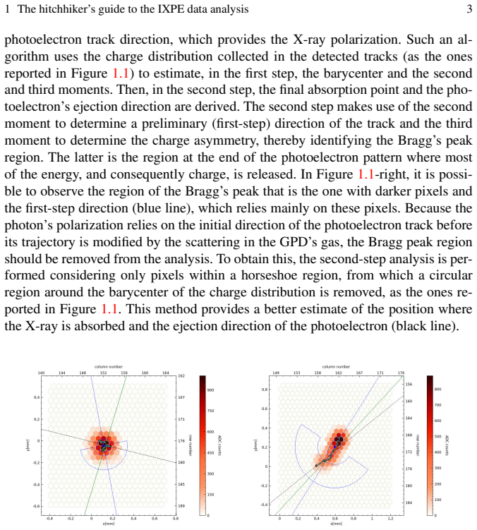
The central machinery is the event-by-event Stokes parameterization of photoelectron tracks (a named identity: each track azimuth is converted to Stokes parameters, so polarization becomes additive and Gaussian). It does the work of making the measurement treatable with standard flux statistics, enabling spectral decomposition and systematic-error removal. Two ingredients carry the optimization: the α^0.75 ellipticity weighting, which the paper states gives the best polarimetric sensitivity, and the spurious-modulation correction maps. In the appendix the new machinery is an empirical pair of energy-dependent background thresholds fitted to a single calibration observation.
Load-bearing premise
The new background thresholds were fitted to a single case study (observation 04252301) and are then assumed to hold for all post-anomaly IXPE data, across energies, intensities, and sky regions; if the DU2 anomaly's effects on track shape vary with time or source brightness, these fixed cuts could misclassify source events as background or vice versa.
What would settle it
Take a bright, highly polarized source observed after the anomaly (for example the Crab nebula) and analyze it twice: once with the new cuts (Eqs. 1.21–1.22) and once with the old pre-anomaly cuts. If the new cuts remove a significant fraction of source events—seen as a drop in the measured source rate or effective area, or a shift in polarization angle—or if an unpolarized source shows non-zero polarization after the new cuts, then the fitted thresholds are not universal.
If this is right
- All IXPE observations analyzed with unweighted or differently weighted Stokes parameters can be re-analyzed with α^0.75 weights to gain roughly 13% in sensitivity.
- Post-anomaly IXPE data reduced with the pre-anomaly background cuts should be reprocessed, because the new cuts remove a class of events that otherwise mimic polarization.
- The background cuts must be applied to bright sources as well, where background subtraction would normally be skipped, to avoid the anomalous low-energy events.
- Using the prescribed source/background region radii (30–100 arcsec source, 150–300 arcsec annulus background) along with the new cuts keeps the measured polarization free of the known detector-edge systematics.
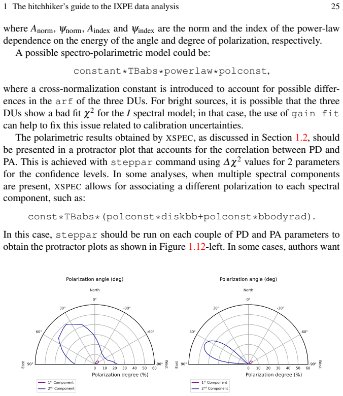
- Polarization detection claims should be judged against the reported P/σ_P thresholds (99%, 99.9%, 99.99%) and presented as 2-D protractor plots, since 1-D errors ignore the P–φ correlation.
Where Pith is reading between the lines
- If the DU2 anomaly's effect on track morphology drifts with time, temperature, or count rate, the fitted thresholds in the appendix may need periodic re-fitting; a simple test would be to track the background/source separation efficiency across multiple post-anomaly observations.
- The success of the α^0.75 weighting suggests that other track-shape statistics (for example, the Bragg-peak asymmetry used in track reconstruction) could be combined into a multivariate weight to push sensitivity further, which could be tested with the mission's simulator.
- The requirement to apply new cuts even to bright sources implies that bright-source polarimetry published from the affected period should be revisited for possible bias; the paper itself does not state this retroactive implication explicitly.
- A publicly reproducible calibration observation, extended to several targets with different brightnesses, would convert the single-case-study thresholds into a validated generic prescription.
Editorial analysis
A structured set of objections, weighed in public.
Referee Report
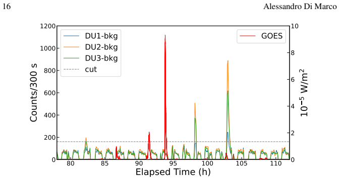
Summary. This book-style chapter is a practical guide to the analysis of IXPE X-ray polarimetric data. It opens with the event-by-event Stokes formalism (Eqs. 1.2–1.9), including spurious-modulation subtraction (Eq. 1.3), the α^0.75 track-ellipticity weighting (Eq. 1.4), and the associated uncertainty, correlation, and MDP99 expressions (Eqs. 1.5–1.9). It then covers data retrieval and FITS formats (Sec. 1.3), the IXPE response functions and their unweighted/weighted/gray-filter flavors (Sec. 1.4), and a preprocessing workflow for image alignment, source/background spatial selection, solar-flare time filtering, and particle-background rejection (Sec. 1.5, Eqs. 1.10–1.16). Model-independent analysis (ixpe_protractor, xpbin/PCUBE) and model-dependent spectro-polarimetric analysis in XSPEC with polconst/pollin/polpow are summarized (Secs. 1.6–1.7). The Appendix, the chapter's only substantially new content, prescribes updated background-rejection thresholds for data taken after a GO2 DU2 pixel failure: a number-of-pixels cut (Eqs. 1.20–1.21) and an energy-fraction cut (Eq. 1.22), fitted to observation ID 04252301 and recommended for all post-anomaly observations, including bright sources.
Significance. As a compilation, the chapter serves a useful purpose: the core Stokes statistics are consistent with the published IXPE literature (Kislat et al. 2015; Di Marco et al. 2022; the IXPE statistics note), the software commands are concrete and reproducible, and the practical advice on alignment, solar flares, and protractor plots will help users avoid known pitfalls. The chapter is also transparent in providing χ²/dof values and best-fit parameters for the new thresholds. The DU2 anomaly is a real operational event and the community needs updated background guidance, so the Appendix addresses a genuine need. Its weakness is that the new, universal prescription rests on a single case study with no independent validation, and the chapter itself notes that the anomalous events depend on count rate and detector region. Since the cut sits upstream of every Stokes measurement, this gap is load-bearing rather than cosmetic. With the addition of cross-validation and a demonstration that the cut does not bias polarization measurements for bright sources, the chapter would be a valuable reference.
major comments (2)
- [Appendix, Eqs. (1.20)–(1.22), Figs. 1.13–1.14] The new background thresholds are fitted to a single observation (ID 04252301) and then prescribed for all post-anomaly IXPE data, including bright sources, without independent validation. The Appendix itself states that the anomalous high-EVT_FRA population 'seem[s] to depend on both the spatial region on the detector surface and the counting rate' (text around Fig. 1.14). That dependence is direct evidence against an observation-independent cut: a population whose incidence varies with position and rate cannot be safely removed by a fixed threshold calibrated on one pointing. No cross-validation on other post-anomaly observations is presented, and the threshold functions (Eqs. 1.21–1.22) are adopted as universal requirements. Because this cut is applied upstream of all later analysis, the author should either (i) validate the fixed thresholds on a sample of post-anomaly observations sp
- [Appendix, Eq. (1.22), Fig. 1.14; Sec. 1.5] The recommendation to apply the new rejection to bright sources conflicts with the chapter's own Sec. 1.5 treatment, where bright-source background is deemed negligible (Eq. 1.10 with B/S≈0). For the cut to be safe in that regime, the removed events must be shown to be non-astrophysical and unpolarized; no such check is provided. The high-EVT_FRA signature (>0.9) of the removed events is also a property of compact, low-energy X-ray tracks, so the cut may reject genuine source photons. The author should demonstrate that applying Eqs. (1.21)–(1.22) leaves Q, U, P, and φ0 unchanged (within uncertainties) for a bright source, and quantify the fraction of source events removed. In addition, the operational definition of the energy-fraction cut is ambiguous: at ~1 keV the fitted threshold of Eq. (1.22) is ≈1.03, above the stated '>0.9' removal goal, so the reader cannot tell whether the operat
minor comments (4)
- [Appendix, Eqs. (1.20)–(1.21) vs Fig. 1.13] The χ²/dof values for the nonlinear and linear fits are swapped between the text (0.92 for Eq. 1.20; 0.7 for Eq. 1.21) and the labels in Fig. 1.13-right (nonlinear 0.70, linear 0.92). Please reconcile.
- [Sec. 1.7, NEFF equations] The printed NEFF equations (I = N_eff/T; Q = (N_eff/(TI)) Σ w_k q_k; σQ = (N_eff/(TI)) sqrt(Σ (w_k q_k)^2)) are dimensionally inconsistent as typeset: with I = N_eff/T, the prefactor N_eff/(TI) equals 1, leaving Q with units of counts rather than flux. If this is a typesetting artifact, please restore the forms from Ref. [17]/the IXPE statistics note, since readers will use these formulas to validate the extraction tools.
- [Sec. 1.5, background rejection; Appendix] It should be stated explicitly that the new post-anomaly cuts (Eqs. 1.20–1.22) replace the pre-anomaly conditions (Eqs. 1.12–1.13) rather than being applied in addition to them; as written, a user could apply both and reject the entire source track population between the two thresholds.
- [Sec. 1.2, Eq. (1.6)] The correlation coefficient in Eq. (1.6) is garbled in typesetting (the denominator is hard to read); please check it against Ref. [17]. The prose statement that ρ is maximized at φ0 = −22.5° with value P²/3 is consistent with the formula for μ=1, but as printed the equation cannot be verified.
Circularity Check
No circularity: the chapter compiles standard IXPE methods and empirically fits thresholds; it does not present fitted quantities as derived predictions.
full rationale
The chapter is an instructional guide, not a derivation that reduces outputs to inputs. The Stokes/weighting formalism (Eqs. 1.2-1.9) restates standard method definitions and results from prior independent publications (Kislat 2015; Di Marco et al. 2022), which are externally grounded; self-citation is present but not circular. The only original quantitative content is the Appendix's new post-anomaly background thresholds (Eqs. 1.21-1.22). These are explicitly fitted to observation 04252301 and presented as empirical tuning ('observation ID 04252301 is considered as a case study'), not as predictions derived from the fit. The chapter itself flags a generalization risk in the same appendix: the anomalous high-EVT_FRA population 'seem[s] to depend on both the spatial region on the detector surface and the counting rate', so applying fixed cuts to all observations may be unsafe; however, that is an overfitting/validation concern, not a circularity. No equation in the paper is equivalent by construction to the quantity it is claimed to predict.
Axiom & Free-Parameter Ledger
free parameters (4)
- k_a, k_b, k_c for number-of-pixels threshold (Eq. 1.20) =
90±6, 26±4, 1.20±0.08
- Linear number-of-pixels cut (Eq. 1.21) =
intercept 76±5, slope 40.8±1.5 per keV
- k_a, k_b, k_c, k_d for energy-fraction threshold (Eq. 1.22) =
0.71±0.05, 0.21±0.07 keV, 1.5±0.2 keV, 0.0012±0.0006 keV^-1
- Weight exponent for event weighting =
0.75
axioms (7)
- domain assumption Photoelectric absorption dominates and its angular distribution follows Eq. 1.1
- domain assumption The GPD track reconstruction recovers the initial photoelectron direction with the accuracy assumed
- domain assumption Spurious-modulation calibration maps fully correct detector systematics (Ref. [22])
- domain assumption Background events in the source region are unpolarized
- domain assumption IRFs (arf, rmf, mrf, vignetting, PSF, modulation factor) represent the instrument over each validity interval
- ad hoc to paper New threshold functions fitted to observation 04252301 generalize to all post-anomaly DU2 data
- standard math Stokes parameters from the weighted analysis follow Gaussian statistics with errors from Eqs. 1.5–1.9
read the original abstract
This chapter provides an almost comprehensive guide to the Imaging X-ray Polarimetry Explorer (IXPE) data analysis. The chapter briefly introduces the IXPE spacecraft and the instrument onboard; subsequently, the strategies adopted to extract polarimetric information and to optimize the response are given. Moreover, the data formats and processing steps to avoid potential systematic errors and to achieve the best results from the IXPE data are reported. Both the model-independent and the model-dependent analyses are summarized, as the instrument response functions and their different available flavors. The idea behind this chapter is to collect suggestions and answers to questions that are typically raised by users, aiming to enable researchers to maximize the scientific return from IXPE observations.
Figures






Forward citations
Cited by 2 Pith papers
-
Peering through the dip: IXPE unveils the extended scattering environment of GX 13+1
During the periodic dip of GX 13+1, X-ray polarization rises to 9.1%±1.1% and rotates by ~60° relative to the off-dip state, consistent with scattering in an oblate corona or disk wind.
-
Unchanged X-Ray Polarization During Accretion Dips in the Low Hard State of Cygnus X-1
During Cygnus X-1 accretion dips the 2–8 keV polarization is unchanged within errors, indicating the absorbed disk does not contribute and supporting an extended oblate corona.
Reference graph
Works this paper leans on
-
[1]
The Instrument of the Imaging X-Ray Polarimetry Explorer,
P. Soffitta, L. Baldini,et al., “The Instrument of the Imaging X-Ray Polarimetry Explorer,” AJ162no. 5, (Nov., 2021) 208,arXiv:2108.00284 [astro-ph.IM]
Pith/arXiv arXiv 2021
-
[2]
The Imaging X-Ray Polarimetry Explorer (IXPE): Pre-Launch,
M. C. Weisskopf, P. Soffitta,et al., “The Imaging X-Ray Polarimetry Explorer (IXPE): Pre-Launch,”JATIS8no. 2, (Apr., 2022) 026002,arXiv:2112.01269 [astro-ph.IM]
Pith/arXiv arXiv 2022
-
[3]
Design, construction, and test of the Gas Pixel Detectors for the IXPE mission,
L. Baldini, M. Barbanera,et al., “Design, construction, and test of the Gas Pixel Detectors for the IXPE mission,”Astroparticle Physics133(Dec., 2021) 102628, arXiv:2107.05496 [astro-ph.IM]
Pith/arXiv arXiv 2021
-
[4]
Heitler,Quantum theory of radiation
W. Heitler,Quantum theory of radiation. International Series of Monographs on Physics, Oxford: Clarendon, 1954
1954
-
[5]
Calibration of the IXPE Focal Plane X-Ray Polarimeters to Polarized Radiation,
A. Di Marco, S. Fabiani,et al., “Calibration of the IXPE Focal Plane X-Ray Polarimeters to Polarized Radiation,” AJ164no. 3, (Sept., 2022) 103,arXiv:2206.07582 [astro-ph.IM]
Pith/arXiv arXiv 2022
-
[6]
D. A. Prokhorov, Y .-J. Yang,et al., “Evidence for a shock-compressed magnetic field in the northwestern rim of Vela Jr. from X-ray polarimetry,” A&A692(Dec., 2024) A59, arXiv:2410.20582 [astro-ph.HE]
Pith/arXiv arXiv 2024
-
[7]
Vela pulsar wind nebula X-rays are polarized to near the synchrotron limit,
F. Xie, A. Di Marco,et al., “Vela pulsar wind nebula X-rays are polarized to near the synchrotron limit,” Nature612no. 7941, (Dec., 2022) 658–660,arXiv:2303.12437 [astro-ph.HE]
Pith/arXiv arXiv 2022
-
[8]
Polarized x-rays constrain the disk-jet geometry in the black hole x-ray binary Cygnus X-1,
H. Krawczynski, F. Muleri,et al., “Polarized x-rays constrain the disk-jet geometry in the black hole x-ray binary Cygnus X-1,”Science378no. 6620, (Nov., 2022) 650–654, arXiv:2206.09972 [astro-ph.HE]
Pith/arXiv arXiv 2022
-
[9]
Weakly Magnetized Accreting Neutron Stars as Seen by IXPE,
A. Di Marco, “Weakly Magnetized Accreting Neutron Stars as Seen by IXPE,” Astronomische Nachrichten346no. 1, (Jan., 2025) e20240126
2025
-
[10]
F. La Monaca, A. Di Marco,et al., “Highly Significant Detection of X-Ray Polarization from the Brightest Accreting Neutron Star Sco X-1,” ApJ960no. 2, (Jan., 2024) L11, arXiv:2311.06359 [astro-ph.HE]
Pith/arXiv arXiv 2024
-
[11]
M. C. Baglio, F. Coti Zelati,et al., “Polarized Multiwavelength Emission from Pulsar Wind—Accretion Disk Interaction in a Transitional Millisecond Pulsar,” ApJ987no. 1, (July, 2025) L19,arXiv:2412.13260 [astro-ph.HE]
Pith/arXiv arXiv 2025
-
[12]
Determination of X-ray pulsar geometry with IXPE polarimetry,
V . Doroshenko, J. Poutanen,et al., “Determination of X-ray pulsar geometry with IXPE polarimetry,”Nature Astronomy6(Dec., 2022) 1433–1443,arXiv:2206.07138 [astro-ph.HE]
Pith/arXiv arXiv 2022
-
[13]
X-Ray Dips and Polarization Angle Swings in GX 13+1,
A. Di Marco, F. La Monaca,et al., “X-Ray Dips and Polarization Angle Swings in GX 13+1,” ApJ979no. 2, (Feb., 2025) L47,arXiv:2501.05511 [astro-ph.HE]
Pith/arXiv arXiv 2025
-
[14]
Discovery of polarized X-ray emission from the accreting millisecond pulsar SRGA J144459.2–604207,
A. Papitto, A. Di Marco,et al., “Discovery of polarized X-ray emission from the accreting millisecond pulsar SRGA J144459.2–604207,” A&A694(Feb., 2025) A37, arXiv:2408.00608 [astro-ph.HE]
Pith/arXiv arXiv 2025
-
[15]
D. E. Kim, L. Di Gesu,et al., “Magnetic field properties inside the jet of Mrk 421. Multiwavelength polarimetry, including the Imaging X-ray Polarimetry Explorer,” A&A681 (Jan., 2024) A12,arXiv:2310.06097 [astro-ph.HE]
Pith/arXiv arXiv 2024
-
[16]
The X-ray polarization of the Seyfert 1 galaxy IC 4329A,
A. Ingram, M. Ewing,et al., “The X-ray polarization of the Seyfert 1 galaxy IC 4329A,” MNRAS525no. 4, (Nov., 2023) 5437–5449,arXiv:2305.13028 [astro-ph.HE]
Pith/arXiv arXiv 2023
-
[17]
A. Di Marco, E. Costa,et al., “A weighted analysis to improve the x-ray polarization sensitivity of the imaging x-ray polarimetry explorer,” AJ163no. 4, (Mar, 2022) 170. https://dx.doi.org/10.3847/1538-3881/ac51c9
-
[18]
Handling the Background in IXPE Polarimetric Data,
A. Di Marco, P. Soffitta,et al., “Handling the Background in IXPE Polarimetric Data,” AJ 165no. 4, (Apr., 2023) 143,arXiv:2302.02927 [astro-ph.IM]
Pith/arXiv arXiv 2023
-
[19]
Novel gaseus X-ray polarimeter: data analysis and simulation,
R. Bellazzini, F. Angelini,et al., “Novel gaseus X-ray polarimeter: data analysis and simulation,” inPolarimetry in Astronomy, S. Fineschi, ed., vol. 4843 ofSociety of Photo-Optical Instrumentation Engineers (SPIE) Conference Series, pp. 383–393. Feb., 2003. 30 Alessandro Di Marco
2003
-
[20]
On the statistical analysis of x-ray polarization measurements,
T. E. Strohmayer and T. R. Kallman, “On the statistical analysis of x-ray polarization measurements,”The Astrophysical Journal773no. 2, (Jul, 2013) 103. https://doi.org/10.1088/0004-637X/773/2/103
-
[21]
Analyzing the data from x-ray polarimeters with stokes parameters,
F. Kislat, B. Clark, M. Beilicke, and H. Krawczynski, “Analyzing the data from x-ray polarimeters with stokes parameters,”Astroparticle Physics68(2015) 45–51.https: //www.sciencedirect.com/science/article/pii/S092765051500033X
2015
-
[22]
J. Rankin, F. Muleri,et al., “An Algorithm to Calibrate and Correct the Response to Unpolarized Radiation of the X-Ray Polarimeter Onboard IXPE,” AJ163no. 2, (Feb., 2022) 39,arXiv:2111.14867 [astro-ph.IM]
Pith/arXiv arXiv 2022
-
[23]
X-Ray Spectro-polarimetry with Photoelectric Polarimeters,
T. E. Strohmayer, “X-Ray Spectro-polarimetry with Photoelectric Polarimeters,” ApJ838 no. 1, (Mar., 2017) 72,arXiv:1703.00949 [astro-ph.IM]
Pith/arXiv arXiv 2017
-
[24]
On understanding the figures of merit for detection and measurement of x-ray polarization,
M. C. Weisskopf, R. F. Elsner, and S. L. O’Dell, “On understanding the figures of merit for detection and measurement of x-ray polarization,” inSpace Telescopes and Instrumentation 2010: Ultraviolet to Gamma Ray, M. Arnaud, S. S. Murray, and T. Takahashi, eds., vol. 7732 ofSociety of Photo-Optical Instrumentation Engineers (SPIE) Conference Series, p. 773...
Pith/arXiv arXiv 2010
-
[25]
Polarisation leakage due to errors in track reconstruction in gas pixel detectors,
N. Bucciantini, N. Di Lalla, R. W. R. Romani, S. Silvestri, M. Negro, L. Baldini, A. F. Tennant, and A. Manfreda, “Polarisation leakage due to errors in track reconstruction in gas pixel detectors,” A&A672(Apr., 2023) A66,arXiv:2302.00346 [astro-ph.IM]
Pith/arXiv arXiv 2023
-
[26]
A study of background for IXPE,
F. Xie, R. Ferrazzoli, P. Soffitta, S. Fabiani, E. Costa, F. Muleri, and D. Marco, “A study of background for IXPE,”Astroparticle Physics128(Mar., 2021) 102566, arXiv:2102.06475 [astro-ph.IM]
Pith/arXiv arXiv 2021
-
[27]
The future of X-ray polarimetry towards the 3-dimensional photoelectron track reconstruction,
D. E. Kim, A. Di Marco,et al., “The future of X-ray polarimetry towards the 3-dimensional photoelectron track reconstruction,”Journal of Instrumentation19no. 2, (Feb., 2024) C02028,arXiv:2309.17206 [astro-ph.IM]
Pith/arXiv arXiv 2024
-
[28]
In-flight calibration system of imaging x-ray polarimetry explorer,
R. Ferrazzoli, F. Muleri,et al., “In-flight calibration system of imaging x-ray polarimetry explorer,”JATIS6(Oct., 2020) 048002,arXiv:2010.14185 [astro-ph.IM]
Pith/arXiv arXiv 2020
-
[29]
ixpeobssim: A simulation and analysis framework for the imaging X-ray polarimetry explorer,
L. Baldini, N. Bucciantini, N. D. Lalla, S. Ehlert, A. Manfreda, M. Negro, N. Omodei, M. Pesce-Rollins, C. Sgr`o, and S. Silvestri, “ixpeobssim: A simulation and analysis framework for the imaging X-ray polarimetry explorer,”SoftwareX19(July, 2022) 101194, arXiv:2203.06384 [astro-ph.IM]
Pith/arXiv arXiv 2022
-
[30]
Optics for the imaging x-ray polarimetry explorer,
B. D. Ramsey, S. D. Bongiorno,et al., “Optics for the imaging x-ray polarimetry explorer,” Journal of Astronomical Telescopes, Instruments, and Systems8(Apr., 2022) 024003
2022
-
[31]
IXPE DU-FM ions-UV filters characterization,
F. La Monaca, S. Fabiani,et al., “IXPE DU-FM ions-UV filters characterization,” inSociety of Photo-Optical Instrumentation Engineers (SPIE) Conference Series, J.-W. A. den Herder, S. Nikzad, and K. Nakazawa, eds., vol. 11444 ofSociety of Photo-Optical Instrumentation Engineers (SPIE) Conference Series, p. 1144463. Jan., 2021
2021
-
[32]
In-orbit monitoring of the imaging x-ray polarimeters on-board IXPE,
A. Di Marco, F. Muleri,et al., “In-orbit monitoring of the imaging x-ray polarimeters on-board IXPE,” inSpace Telescopes and Instrumentation 2022: Ultraviolet to Gamma Ray, J.-W. A. den Herder, S. Nikzad, and K. Nakazawa, eds., vol. 12181 ofSociety of Photo-Optical Instrumentation Engineers (SPIE) Conference Series, p. 121811C. Aug., 2022
2022
-
[33]
Simultaneous space and phase resolved X-ray polarimetry of the Crab pulsar and nebula,
N. Bucciantini, R. Ferrazzoli,et al., “Simultaneous space and phase resolved X-ray polarimetry of the Crab pulsar and nebula,”Nature Astronomy7(May, 2023) 602–610, arXiv:2207.05573 [astro-ph.HE]
Pith/arXiv arXiv 2023
-
[34]
IXPE Observations of the Quintessential Wind-accreting X-Ray Pulsar Vela X-1,
S. V . Forsblom, J. Poutanen,et al., “IXPE Observations of the Quintessential Wind-accreting X-Ray Pulsar Vela X-1,” ApJ947no. 2, (Apr., 2023) L20,arXiv:2303.01800 [astro-ph.HE]
Pith/arXiv arXiv 2023
-
[35]
A polarized view of the young pulsar wind nebula 3C 58 with IXPE,
N. Bucciantini, J. Wong,et al., “A polarized view of the young pulsar wind nebula 3C 58 with IXPE,” A&A699(June, 2025) A33,arXiv:2504.20534 [astro-ph.HE]
Pith/arXiv arXiv 2025
-
[36]
First X-Ray Polarimetric View of a Low-luminosity Active Galactic Nucleus: The Case of NGC 2110,
S. Chakraborty, A. Ratheesh,et al., “First X-Ray Polarimetric View of a Low-luminosity Active Galactic Nucleus: The Case of NGC 2110,” ApJ990no. 1, (Sept., 2025) 89, arXiv:2503.01071 [astro-ph.HE]. 1 The hitchhiker’s guide to the IXPE data analysis 31
Pith/arXiv arXiv 2025
-
[37]
Magnetic-field Order in the Southwestern Rim of RCW 86 Constrained Using X-Ray Polarimetry,
S. Silvestri, D. Prokhorov,et al., “Magnetic-field Order in the Southwestern Rim of RCW 86 Constrained Using X-Ray Polarimetry,” ApJ998no. 1, (Feb., 2026) 172, arXiv:2602.19200 [astro-ph.HE]
arXiv 2026
-
[38]
XSPEC: The First Ten Years,
K. A. Arnaud, “XSPEC: The First Ten Years,” inAstronomical Data Analysis Software and Systems V, G. H. Jacoby and J. Barnes, eds., vol. 101 ofASP Conf. Ser ., pp. 17–20. Astron. Soc. Pac., San Francisco, 1996
1996
discussion (0)
Sign in with ORCID, Apple, or X to comment. Anyone can read and Pith papers without signing in.