REVIEW 3 major objections 6 minor 1 cited by
A hybrid stabilizer–tensor-network simulator is the better classical choice for Clifford-heavy circuits with moderate non-Clifford content.
Reviewed by Pith at T0; open to challenge. T0 means a machine referee read the full paper against a public rubric. the ladder, T0–T4 →
T0 review · grok-4.5
2026-07-31 19:49 UTC pith:7LVWL6Z5
load-bearing objection Clean open implementation of Mello’s HSMPO plus a usable cost/fidelity map; the Fig. 5 “preferred” region rests on assumed χ ratios that the benchmarks never invert. the 3 major comments →
MPStab: an hybrid stabilizers tensor-network quantum circuit simulator
The pith
A machine-rendered reading of the paper's core claim, the machinery that carries it, and where it could break.
Core claim
For circuits dominated by Clifford gates and interspersed with a moderate number of non-Clifford rotations, the hybrid stabilizer-MPO method reaches higher fidelity than pure matrix-product-state simulation at fixed bond dimension and is cheaper in the low-non-Clifford, high-Clifford region of the cost landscape; the analytical cost model matches the measured wall-clock crossover against a pure tensor-network engine.
What carries the argument
Hybrid stabilizer-MPO (HSMPO) decomposition: conjugate Clifford blocks through local magic rotations so each dressed rotation remains an exact bond-2 MPO; evolve observables exactly with stabilizer tableau arithmetic and apply the dressed rotations approximately to a truncated MPS of bond dimension χ.
Load-bearing premise
That the controlled benchmark family (tunable magic fraction plus CNOT ladders) and the bond-dimension savings seen there are representative of the real circuits where the method would be preferred.
What would settle it
On the same Clifford-heavy, moderate-magic circuits, run the hybrid method and a pure tensor-network engine at identical bond dimension and contraction settings; if the hybrid method does not show higher fidelity lower bounds and the measured time crossover fails to track the analytical cost-ratio contour, the central performance claim is false.
If this is right
- Near-Clifford surrogate circuits used in learning-based error mitigation can be simulated at larger sizes than pure tensor networks allow while retaining controlled magic.
- The analytical cost map supplies a practical decision rule for choosing hybrid versus pure MPS simulation from gate counts and target bond dimension.
- Modular stabilizer and tensor-network engines can be swapped inside hybrid quantum–classical pipelines that keep the classical side on near-Clifford circuits.
- How Clifford substructure shapes the locality of dressed generators becomes a design lever for keeping bond-dimension growth slow.
Where Pith is reading between the lines
- The same conjugation-plus-bond-2-MPO rewrite can sit in front of other approximate engines (for example sparse Pauli propagation on the observable side) without changing the circuit identity.
- If bond-dimension savings shrink on dense long-range connectivity, the hybrid-favourable region of the cost map may be narrower than the ladder benchmarks suggest.
- Controlled magic retention while Clifford-izing the rest is a natural classical backend for data-driven error mitigation beyond exact state-vector sizes.
Editorial analysis
A structured set of objections, weighed in public.
Referee Report
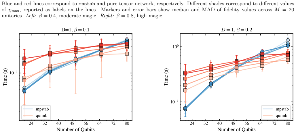
Summary. The manuscript presents mpstab, an open-source Python implementation of the hybrid stabilizer–MPO (HSMPO) simulation framework of Mello et al. [1]. Circuits are decomposed into Clifford blocks (handled exactly via stabilizer tableau backpropagation of the observable) and dressed non-Clifford rotations (applied as exact bond-2 MPOs to an MPS with truncation at bond dimension χ). The paper describes the package architecture (engines/evolutors/models, Qibo integration), derives an analytical cost model for mpstab versus standard MPS simulation (Eqs. 13–14), maps the "preferred simulator" region in the (N_C, N_nC) plane (Fig. 5), and benchmarks against Quimb under matched contraction settings on a controlled ansatz with tunable magic retention β and CNOT-ladder depth (Fig. 6, Eq. 15). Benchmarks show: (i) wall-clock crossover versus pure MPS at the magic fraction predicted by the cost model at L=35 and L=80 (Fig. 7); (ii) systematically higher fidelity lower bounds F_lb = ∥ψ_trunc∥² at fixed χ_max, with the gap widening with depth (Fig. 8); (iii) steeper wall-clock scaling with system size at fixed β (Fig. 9). The authors conclude mpstab is the preferred simulator for Clifford-dominated circuits with moderate non-Clifford content.
Significance. If the results hold, this is a useful contribution: a well-engineered, open-source implementation of a recent PRL formalism, with reproducible benchmarks (M=20 random unitaries, median/MAD statistics, shared contraction backends to exclude implementation asymmetries) and an analytical cost model whose crossover prediction is actually confronted with wall-clock data rather than asserted. The identification of the low-N_nC/high-N_C regime as the method's comfort zone is practically valuable, especially for near-Clifford surrogate generation in error mitigation (Clifford Data Regression), a compelling use case the authors highlight. The fidelity advantage at fixed bond dimension (Fig. 8) is directly demonstrated and is the paper's most solid empirical result. The weaker link is the translation of that fidelity gap into the matched-accuracy bond-dimension ratio on which the phase map of Fig. 5 entirely rests; see Major Comment 1.
major comments (3)
- [§III.D.1, Eqs. (13)–(14), Fig. 5] The phase map of Fig. 5 — the paper's central practical deliverable — is drawn with assumed bond-dimension ratios χ_mps/χ_mpstab ∈ {1.1, 2.5} that are never measured. The text states these 'encode the bond-dimension saving that mpstab achieves at fixed fidelity,' but no benchmark performs the required inversion: what χ_mps does Quimb need to match mpstab's F_lb at a given χ_mpstab? Fig. 8 demonstrates a fidelity gap at *equal* χ_max, which is not the same quantity. Because C_mps scales cubically in χ_mps (Eq. 13), the entire red region is highly sensitive to this ratio: a true matched-fidelity ratio of 1.05 instead of 1.1 shrinks the favorable region substantially, and a ratio at or below 1 — conceivable for circuits whose dressed generators are weight-L Pauli strings injecting entanglement across every cut simultaneously — would invert the conclusion. The fix is within the manuscript's
- [§IV.A.b, Eq. (16), Fig. 8] The accuracy certificate F_lb = ∥ψ_trunc∥² is a rigorous lower bound on state fidelity, but mpstab's product is expectation values, and equal norm retention does not imply equal |⟨O⟩| error: two truncated states with identical F_lb can differ substantially in observable error, depending on how the discarded Schmidt weight aligns with O. Since the whole 'preferred simulator' argument is about expectation-value accuracy at matched cost, the paper should establish that F_lb rankings track observable-error rankings. This is feasible: for small L (e.g., L=20 in Table I, within statevector reach) report the actual |⟨O⟩_mpstab − ⟨O⟩_exact| and |⟨O⟩_Quimb − ⟨O⟩_exact| alongside F_lb for the same circuits, and confirm the ordering. Without this, the conclusion of §IV.B.d rests on an unverified proxy.
- [§IV.B.a, Fig. 7] The cost-model validation — which licenses trusting Fig. 5 'as a practical guide' — consists of crossover agreement at exactly two points (L=35 and L=80, both at D=1 and a single (β,k) ansatz family). The predicted crossover values (42.86% and 18.75%) are stated to fall 'inside the interval where the measured curves actually cross,' but the width of that interval is not quantified, and no validation is offered at D>1, where the N_nC·N_C dressing term and accumulated truncation may shift the balance. Given that this validation is the empirical anchor for the entire cost-model narrative, at minimum the crossover uncertainty (from the M=20 repetitions) should be reported, and ideally one depth-2 or depth-3 configuration should be added to show the agreement is not specific to D=1.
minor comments (6)
- [§III.D, Eq. (13)] The standard-MPS cost C_mps assumes worst-case interaction range ℓ=L for all N gates. For circuits with predominantly nearest-neighbor entanglers this overestimates C_mps and tilts the comparison in mpstab's favor; the benchmark ansatz does contain long-range CNOTs, so the benchmarks are unaffected, but the cost map's generality should be qualified with a sentence on how the boundary moves for ℓ ≪ L.
- [§IV, Fig. 7 caption] The caption labels the vertical line 'C_tn/C_mpstab = 1' while the text and Eqs. (13)–(14) use C_mps; please make the notation consistent. Also, both panels say 'varying bond dimensions' but the figure does not indicate which χ_max (or χ for each method) is used — state it explicitly.
- [§II.A, below Eq. (6)] Typos: 'adressing' → 'addressing'; §II.C 'corresponing' → 'corresponding'; §IV opening 'pletora' → 'plethora'; Fig. 1 caption and §I 'consent simulation' → 'allow/enable simulation'; §I 'bijector of the plane' is unusual — 'diagonal' is presumably meant.
- [§III.A, first code snippet] The snippet calls CZ(0,3) and CZ(4,1) without the gates. prefix used on the preceding line; as written it will not run. Also 'H a r d w a r e E f f i c i e n t' and similar spacing artifacts suggest the listings were not typeset from the actual source.
- [§III.D.b] The complexity derivation quotes the SVD cost as O(d D³ χ³) per site with prefactor 16 retained in Eq. (14), but the MPO application cost O(16 L χ²) uses D=2 while the backpropagated observable in step (c) is a bond-1 product operator — the prefactor bookkeeping between contraction and compression steps could be made uniform, or prefactors dropped consistently throughout.
- [References] Refs. [15] and [20] are the same Stim paper (C. Gidney, Quantum 5, 497 (2021)) cited twice; please merge. Consider also citing related stabilizer–tensor-network benchmarks beyond [19, 21] to situate the fidelity-at-fixed-χ comparison.
Circularity Check
No significant circularity: HSMPO is an external construction; cost map and benchmarks are independent comparisons, not self-forced predictions.
full rationale
The paper implements the hybrid stabilizer-MPO formalism of Mello et al. [1] (an external PRL) and packages it as mpstab. The analytical cost model (Eqs. 13–14) is derived from standard gate-count and bond-dimension scalings; the phase map of Fig. 5 is an explicit parametric exploration over assumed ratios χ_mps/χ_mpstab ∈ {1.1, 2.5}, not a fit to data that is then re-presented as a prediction. Benchmarks compare wall-clock time and a fidelity lower bound against an independent Quimb baseline under matched contraction settings; the Fig. 7 crossover check is a consistency test of the cost formulas, not a circular recovery of fitted parameters. Self-references are to the authors’ repository, docs, and Qibo ecosystem integrations—none of which supply a uniqueness theorem or an equation that already equals the claimed preferred-simulator regime. The skeptic’s concern that the matched-accuracy χ ratio is assumed rather than measured is a validity/transfer gap, not a circular reduction of outputs to inputs. Score 1 for ordinary self-citation of tooling only.
Axiom & Free-Parameter Ledger
free parameters (3)
- χ_mps/χ_mpstab ratio in cost phase map =
1.1 and 2.5 (illustrative)
- Benchmark magic retention β and ladder cutoff k =
β ∈ {0..1}; k illustrated at 5 in Fig. 6
- Maximum MPS bond dimension χ_max =
2–32 in benchmarks
axioms (6)
- standard math Aaronson–Gottesman: Clifford evolution of Pauli observables via tableau is exact and poly-time (O(N_C L) scale used in the paper).
- standard math Any Pauli-string rotation exp(-iθΣ_γ/2) admits an exact bond-dimension-2 MPO (Eqs. 7–9).
- domain assumption Any universal circuit decomposes as alternating Clifford blocks and local Pauli-axis rotations (Eq. 1), so Cliffords can be pushed through by conjugation (Eqs. 5–6).
- domain assumption Truncation error is faithfully monitored by the MPS norm fidelity lower bound F_lb=∥ψ_trunc∥² under unitary evolution (Eq. 16).
- domain assumption HSMPO mixed-picture evolution as introduced in Mello et al. [1] is the correct target semantics for the package.
- ad hoc to paper Cost model worst-case interaction range ℓ=L and O(L) Pauli terms in the observable for C_mps and C_mpstab (Eqs. 13–14).
invented entities (1)
-
mpstab HSMPO evolutor package (engines/evolutors/models modules)
independent evidence
read the original abstract
The development of techniques for simulating quantum systems using classical computers is a paramount task for two primary reasons: i) there exist configurations for which classical computers are remarkably effective and will continue to be so, and ii) exploring the limits of classical computation facilitates the identification of the regimes of competence for quantum computers. In this work, we present MPStab, a quantum circuit simulator based on a hybrid formalism combining stabilizers and tensor networks, recently introduced in Ref. [1]. We present the package, its core functionalities, and explore its performances in a few interesting simulation regimes.
Figures


Forward citations
Cited by 1 Pith paper
-
SymFT: Universal Fault-Tolerant Quantum Circuit Simulation via Symbolic Clifford--Pauli Frames and Stabilizer Coordinates
SymFT reaches state-of-the-art exact sampling of Clifford-dominated FT circuits by combining symbolic Clifford–Pauli frames with planned dense stabilizer-coordinate updates.
Reference graph
Works this paper leans on
-
[1]
Comparison with standard MPS 7 IV. Benchmarks 8 A. Benchmark setup 8 B. Numerical results 9 V. Conclusions 11 VI. Acknowledgments 12 References 12 I. INTRODUCTION Simulating quantum systems on classical computers is a fundamental challenge in quantum information sci- ence. The most straightforward approach, statevector simulation, represents the quantum s...
Pith/arXiv arXiv 2026
-
[2]
pushed through
followed by a Hadamard on qubits 0 and 2, the gener- ator transforms under conjugation as IIZII CNOT02 − − − − − →ZIZII H0⊗H2 − − − − − →XIXII,(4) whereZon the target backpropagates to the control qubit viaZ t →Z cZt, andHZH † =Xmaps each remain- ingZtoX. The originally local rotation exp(−iθ Z 2/2) is thus conjugated into the genuinely non-local two-body...
-
[3]
fidelity
Comparison with standard MPS In standard matrix product state (MPS) simulation, gates are applied sequentially to the state representation. As discussed in [27], single-qubit gates can be applied to an MPS state with costO(χ 2), adjacent two-qubit gates with costO(χ 3), and non-adjacent two-qubit gates acting across spatial distancerrequire swap sequences...
2022
-
[4]
A. F. Mello, A. Santini, and M. Collura, Physical Review Letters133, 10.1103/physrevlett.133.150604 (2024)
-
[5]
A. Javadi-Abhari, M. Treinish, K. Krsulich, C. J. Wood, J. Lishman, J. Gacon, S. Martiel, P. D. Nation, L. S. Bishop, A. W. Cross, B. R. Johnson, and J. M. Gambetta, Quantum computing with Qiskit (2024), arXiv:2405.08810 [quant-ph]
Pith/arXiv arXiv 2024
-
[6]
Developers, Cirq (2025)
C. Developers, Cirq (2025)
2025
-
[7]
V. Bergholm, J. Izaac, M. Schuld, C. Gogolin, S. Ahmed, V. Ajith, M. S. Alam, G. Alonso-Linaje, B. Akash- Narayanan, A. Asadi, J. M. Arrazola, U. Azad, S. Ban- ning, C. Blank, T. R. Bromley, B. A. Cordier, J. Ceroni, A. Delgado, O. D. Matteo, A. Dusko, T. Garg, D. Guala, A. Hayes, R. Hill, A. Ijaz, T. Isacsson, D. Ittah, S. Ja- hangiri, P. Jain, E. Jiang,...
Pith/arXiv arXiv 2022
-
[8]
Efthymiou, S
S. Efthymiou, S. Ramos-Calderer, C. Bravo-Prieto, A. P´ erez-Salinas, D. Garc ´ ıa-Mart ´ ın, A. Garcia-Saez, J. I. Latorre, and S. Carrazza, Quantum Science and Technol- ogy7, 015018 (2021)
2021
-
[9]
Suzuki, Y
Y. Suzuki, Y. Kawase, Y. Masumura, Y. Hiraga, M. Nakadai, J. Chen, K. M. Nakanishi, K. Mitarai, R. Imai, S. Tamiya, T. Yamamoto, T. Yan, T. Kawakubo, Y. O. Nakagawa, Y. Ibe, Y. Zhang, H. Yamashita, H. Yoshimura, A. Hayashi, and K. Fujii, Quantum5, 559 (2021)
2021
-
[10]
Efthymiou, M
S. Efthymiou, M. Lazzarin, A. Pasquale, and S. Carrazza, Quantum6, 814 (2022)
2022
-
[11]
M. Tejedor, B. Casas, J. Conejero, A. Cervera-Lierta, and R. M. Badia, Distributed quantum circuit cutting for hybrid quantum-classical high-performance comput- ing (2025), arXiv:2505.01184 [cs.DC]
Pith/arXiv arXiv 2025
-
[12]
Or´ us, Annals of Physics349, 117–158 (2014)
R. Or´ us, Annals of Physics349, 117–158 (2014)
2014
-
[13]
Gray, Journal of Open Source Software3, 819 (2018)
J. Gray, Journal of Open Source Software3, 819 (2018)
2018
-
[14]
Fishman, S
M. Fishman, S. R. White, and E. M. Stoudenmire, Sci- Post Phys. Codebases , 4 (2022)
2022
-
[15]
J. Hauschild and F. Pollmann, SciPost Physics Lecture Notes 10.21468/scipostphyslectnotes.5 (2018)
-
[16]
Ballarin, F
M. Ballarin, F. P. Barone, A. Coppi, D. Jaschke, S. Mon- tangero, G. M. Men´ es, D. Rattacaso, and N. Reini´ c, Quantum tea: qmatchatea (2025), cite for qmatchatea
2025
-
[17]
S. Aaronson and D. Gottesman, Physical Review A70, 10.1103/physreva.70.052328 (2004)
-
[19]
M. S. Rudolph, T. Jones, Y. Teng, A. Angrisani, and Z. Holmes, Pauli propagation: A computational framework for simulating quantum systems (2025), arXiv:2505.21606 [quant-ph]. 13
Pith/arXiv arXiv 2025
-
[20]
M. L. Goh, M. Larocca, L. Cincio, M. Cerezo, and F. Sauvage, Physical Review Research7, 10.1103/3y65- f5w6 (2025)
-
[21]
H. Lange, A. V. de Walle, A. Abedinnia, and A. Bohrdt, From architectures to applications: A review of neural quantum states (2024), arXiv:2402.09402 [cond-mat.dis- nn]
Pith/arXiv arXiv 2024
-
[22]
S. Masot-Llima and A. Garcia-Saez, Physical Review Let- ters133, 10.1103/physrevlett.133.230601 (2024)
-
[23]
Gidney, Quantum5, 497 (2021)
C. Gidney, Quantum5, 497 (2021)
2021
-
[24]
Beguˇ si´ cet al., Science Advances10, eadk4321 (2024)
T. Beguˇ si´ cet al., Science Advances10, eadk4321 (2024)
2024
-
[25]
T. Haug and L. Piroli, Physical Review B107, 10.1103/physrevb.107.035148 (2023)
-
[26]
addons team, Pauli prop,https://github.com/ Qiskit/pauli-prop(2025)
Q. addons team, Pauli prop,https://github.com/ Qiskit/pauli-prop(2025)
2025
-
[27]
Robbiati, G
M. Robbiati, G. Crognaletti, and M. Robbiano, MPStab docs: qibo backend provider (2024), accessed: 2026-05- 06
2024
-
[28]
M. Robbiati, A. Papaluca, A. Pasquale, E. Pedicillo, R. M. S. Farias, A. Sopena, M. Robbiano, G. Alramahi, S. Bordoni, A. Candido, N. Laurora, J. S. Neto, Y. P. Tan, M. Grossi, and S. Carrazza, Qiboml: towards the or- chestration of quantum-classical machine learning (2025), arXiv:2510.11773 [quant-ph]
arXiv 2025
-
[29]
Efthymiou, A
S. Efthymiou, A. Orgaz-Fuertes, R. Carobene, J. Cereijo, A. Pasquale, S. Ramos-Calderer, S. Bordoni, D. Fuentes- Ruiz, A. Candido, E. Pedicillo, M. Robbiati, Y. P. Tan, J. Wilkens, I. Roth, J. I. Latorre, and S. Carrazza, Quan- tum8, 1247 (2024)
2024
-
[30]
Jozsa, On the simulation of quantum circuits (2006), arXiv:quant-ph/0603163 [quant-ph]
R. Jozsa, On the simulation of quantum circuits (2006), arXiv:quant-ph/0603163 [quant-ph]
Pith/arXiv arXiv 2006
-
[31]
S. Masot-Llima, P. Sierant, P. Stornati, and A. Garcia- Saez, Physical Review B114, 10.1103/5g5b-5rrz (2026)
discussion (0)
Sign in with ORCID, Apple, or X to comment. Anyone can read and Pith papers without signing in.