Technique-agnostic exoplanet demography for the Roman era -- I. Testing a demography retrieval framework using simulated Kepler-like transit datasets
Pith reviewed 2026-05-18 12:52 UTC · model grok-4.3
The pith
The TAED framework enables internally consistent exoplanet demographic forecasts for all detection methods by embedding planetary systems in a galactic stellar population model.
A machine-rendered reading of the paper's core claim, the machinery that carries it, and where it could break.
Core claim
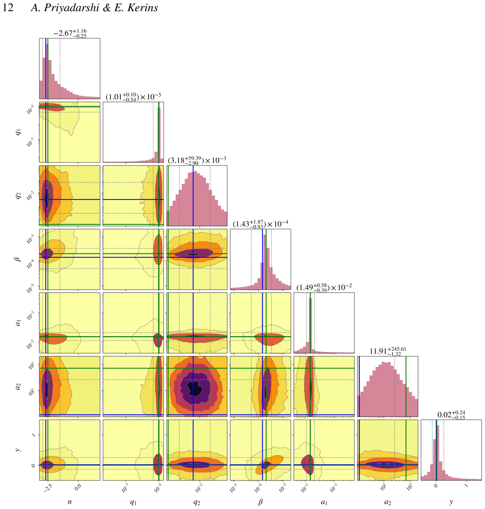
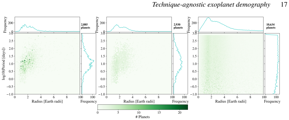
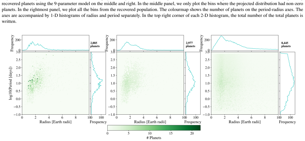
The TAED forward modelling and retrieval framework uses parameterised model exoplanet demographic distributions to embed planetary systems within a stellar population synthesis model of the Galaxy, enabling internally consistent forecasts to be made for all detection methods that are based on spatio-kinematic system properties. In this paper, as a first test of the TAED framework, we apply it to simulated transit datasets based on the Kepler Data Release 25 to assess parameter recovery accuracy and method scalability for a single large homogeneous dataset. We find that optimisation using differential evolution provides a computationally scalable framework that gives a good balance between
What carries the argument
TAED forward modelling and retrieval framework that embeds parameterized exoplanet demographic distributions within a stellar population synthesis model of the Galaxy
Load-bearing premise
The parameterized model exoplanet demographic distributions and the stellar population synthesis model of the Galaxy accurately capture the underlying distributions and selection effects without significant mismatch to real Galactic structure or planet occurrence rates.
What would settle it
A test where the parameters recovered from the simulated Kepler-like datasets significantly deviate from the input values used to create those simulations would show that the retrieval is not accurate.
Figures


read the original abstract
The Nancy Grace Roman Space Telescope (Roman) will unveil for the first time the full architecture of planetary systems across Galactic distances through the discovery of up to 200,000 cool and hot exoplanets using microlensing and transit detection methods. Roman's huge exoplanet haul, and Galactic reach, will require new methods to leverage the full exoplanet demographic content of the combined microlensing and transit samples, given the different sensitivity bias of the techniques to planet and host properties and Galactic location. We present a framework for technique-agnostic exoplanet demography (TAED) that can allow large, multi-technique exoplanet samples distributed over Galactic distance scales to be combined for demographic studies. Our TAED forward modelling and retrieval framework uses parameterised model exoplanet demographic distributions to embed planetary systems within a stellar population synthesis model of the Galaxy, enabling internally consistent forecasts to be made for all detection methods that are based on spatio-kinematic system properties. In this paper, as a first test of the TAED framework, we apply it to simulated transit datasets based on the Kepler Data Release 25 to assess parameter recovery accuracy and method scalability for a single large homogeneous dataset. We find that optimisation using differential evolution provides a computationally scalable framework that gives a good balance between computational efficiency and accuracy of parameter recovery.
Editorial analysis
A structured set of objections, weighed in public.
Referee Report
Summary. The paper introduces the Technique-Agnostic Exoplanet Demography (TAED) framework, which embeds parameterized exoplanet demographic distributions within a stellar population synthesis model of the Galaxy. This enables internally consistent forecasts for exoplanet detection methods (transit, microlensing) based on spatio-kinematic properties, with the goal of supporting combined demographic analyses of Roman Space Telescope data. As a first test, the authors apply the framework to simulated Kepler DR25-like transit datasets and report that differential evolution optimization recovers the input parameters with good accuracy while offering a favorable balance of computational efficiency and scalability.
Significance. If the recovery results hold under the reported conditions, the TAED framework would offer a practical route to unified demographic inference across detection techniques with differing selection biases and Galactic reach. The forward-modeling approach with known-truth simulations provides a clear test of internal consistency, and the adoption of differential evolution is a pragmatic strength for scalability on large datasets. This is a useful foundation for subsequent papers extending the method to microlensing and real Roman data.
major comments (1)
- [Abstract] Abstract: the claim that differential evolution 'gives a good balance between computational efficiency and accuracy of parameter recovery' is not accompanied by quantitative metrics (e.g., fractional bias, credible-interval coverage, or runtime comparisons against alternative optimizers such as MCMC). Without these numbers or a results table/figure showing them, the central claim of the test remains difficult to evaluate.
minor comments (2)
- The manuscript should explicitly state the functional forms and free parameters of the exoplanet demographic distributions (e.g., occurrence-rate slopes, period-radius joint distribution) used in the forward model, ideally with a dedicated methods subsection or table.
- A short forward-looking paragraph on how the same framework will be applied to simulated microlensing datasets would strengthen the technique-agnostic framing, even if detailed results are reserved for Paper II.
Simulated Author's Rebuttal
We thank the referee for their positive assessment of our manuscript and for the constructive comment, which helps us improve the clarity of our central claims. We address the point below and will incorporate revisions in the next version.
read point-by-point responses
-
Referee: [Abstract] Abstract: the claim that differential evolution 'gives a good balance between computational efficiency and accuracy of parameter recovery' is not accompanied by quantitative metrics (e.g., fractional bias, credible-interval coverage, or runtime comparisons against alternative optimizers such as MCMC). Without these numbers or a results table/figure showing them, the central claim of the test remains difficult to evaluate.
Authors: We thank the referee for this observation. The main text (Sections 3 and 4) presents the quantitative results of the differential evolution retrieval on the simulated Kepler DR25-like datasets, including direct comparisons of recovered demographic parameters to the known input values and discussion of the optimization's performance on large samples. We agree that the abstract would benefit from explicit metrics to support the stated balance. In the revised manuscript we will update the abstract to include concise quantitative indicators drawn from the existing results (e.g., typical recovery accuracy and computational scaling), while retaining the paper's focus on framework validation rather than a full optimizer benchmark. Direct runtime comparisons against MCMC are not part of the current analysis, as our goal was to demonstrate internal consistency of the TAED forward model with differential evolution; we can expand the methods discussion to justify this choice if the referee considers it helpful. revision: yes
Circularity Check
No circularity: framework validated via independent simulation benchmarks
full rationale
The paper describes a TAED forward-modeling framework that embeds parameterized exoplanet demographics inside a Galactic stellar population synthesis model to generate technique-agnostic forecasts. Its central test applies the retrieval pipeline to simulated Kepler DR25-like transit datasets whose inputs are known by construction of the simulation. Parameter recovery accuracy is then measured against those known inputs using differential evolution. This is a standard external benchmark test rather than a self-referential loop; the reported success demonstrates optimizer performance when generative assumptions match exactly, without any quoted equation or claim reducing a prediction to a fitted quantity by definition. No load-bearing self-citations, uniqueness theorems, or ansatzes are invoked in the provided text that would collapse the derivation chain.
Axiom & Free-Parameter Ledger
free parameters (1)
- parameters of the exoplanet demographic distributions
axioms (1)
- domain assumption The stellar population synthesis model accurately represents the spatial, kinematic, and stellar properties of the Galaxy.
Lean theorems connected to this paper
-
IndisputableMonolith/Cost/FunctionalEquation.leanwashburn_uniqueness_aczel unclear?
unclearRelation between the paper passage and the cited Recognition theorem.
uses parameterised model exoplanet demographic distributions to embed planetary systems within a stellar population synthesis model of the Galaxy
-
IndisputableMonolith/Foundation/RealityFromDistinction.leanreality_from_one_distinction unclear?
unclearRelation between the paper passage and the cited Recognition theorem.
two-stage broken power law for the number N of planets with planet-star mass ratio q
What do these tags mean?
- matches
- The paper's claim is directly supported by a theorem in the formal canon.
- supports
- The theorem supports part of the paper's argument, but the paper may add assumptions or extra steps.
- extends
- The paper goes beyond the formal theorem; the theorem is a base layer rather than the whole result.
- uses
- The paper appears to rely on the theorem as machinery.
- contradicts
- The paper's claim conflicts with a theorem or certificate in the canon.
- unclear
- Pith found a possible connection, but the passage is too broad, indirect, or ambiguous to say the theorem truly supports the claim.
Reference graph
Works this paper leans on
-
[1]
Astropy Collaboration et al., 2022, @doi [ ] 10.3847/1538-4357/ac7c74 , https://ui.adsabs.harvard.edu/abs/2022ApJ...935..167A 935, 167
work page internal anchor Pith review doi:10.3847/1538-4357/ac7c74 2022
-
[2]
Brown T. M., Latham D. W., Everett M. E., Esquerdo G. A., 2011, @doi [AJ] 10.1088/0004-6256/142/4/112 , 142, 112
-
[3]
Buchner J., 2021, @doi [The Journal of Open Source Software] 10.21105/joss.03001 , https://ui.adsabs.harvard.edu/abs/2021JOSS....6.3001B 6, 3001
-
[4]
Burke C. J., Catanzarite J., 2017, Planet Detection Metrics: Per-Target Detection Contours for Data Release 25 , KSCI-19111-002
work page 2017
-
[5]
J., et al., 2015, @doi [ApJ] 10.1088/0004-637X/809/1/8 , 809, 8
Burke C. J., et al., 2015, @doi [ApJ] 10.1088/0004-637X/809/1/8 , 809, 8
-
[6]
Edmondson K., Norris J., Kerins E., 2023, @doi [arXiv e-prints] 10.48550/arXiv.2310.16733 , https://ui.adsabs.harvard.edu/abs/2023arXiv231016733E p. arXiv:2310.16733
-
[7]
J., et al., 2017, @doi [The Astronomical Journal] 10.3847/1538-3881/aa80eb , 154, 109
Fulton B. J., et al., 2017, @doi [The Astronomical Journal] 10.3847/1538-3881/aa80eb , 154, 109
-
[8]
S., Meyer M., Christiansen J., 2021, in 2514-3433, ExoFrontiers
Gaudi B. S., Meyer M., Christiansen J., 2021, in 2514-3433, ExoFrontiers. IOP Publishing, pp 2--1 to 2--21, @doi 10.1088/2514-3433/ABFA8FCH2
-
[9]
Hsu D. C., Ford E. B., Ragozzine D., Morehead R. C., 2018, @doi [AJ] 10.3847/1538-3881/AAB9A8 , 155, 205
-
[10]
Jeyakumar G., Shanmugavelayutham C., 2011, @doi [International Journal of Artificial Intelligence & Applications] 10.5121/ijaia.2011.2209 , 2, 116–127
-
[11]
Johnson S. A., Penny M., Gaudi B. S., Kerins E., Rattenbury N. J., Robin A. C., Calchi Novati S., Henderson C. B., 2020, @doi [The Astronomical Journal] 10.3847/1538-3881/aba75b , 160, 123
-
[12]
Jordi K., Grebel E. K., Ammon K., 2006, @doi [A&A] 10.1051/0004-6361:20066082 , 460, 339
-
[13]
Marshall D. J., Robin A. C., Reyl \' e C., Schultheis M., Picaud S., 2006, @doi [A&A] 10.1051/0004-6361:20053842 , 453, 635
-
[14]
Montet B. T., Yee J. C., Penny M. T., 2017, @doi [Publications of the Astronomical Society of the Pacific] 10.1088/1538-3873/aa57fb , 129, 044401
-
[15]
D., Pascucci I., Apai D., Ciesla F
Mulders G. D., Pascucci I., Apai D., Ciesla F. J., 2018, @doi [AJ] 10.3847/1538-3881/AAC5EA , 156, 24
-
[16]
Obertas A., Van Laerhoven C., Tamayo D., 2017, @doi [Icarus] https://doi.org/10.1016/j.icarus.2017.04.010 , 293, 52
-
[17]
D., Gould A., Fernandes R., 2018, @doi [ApJ] 10.3847/2041-8213/AAB6AC , 856, L28
Pascucci I., Mulders G. D., Gould A., Fernandes R., 2018, @doi [ApJ] 10.3847/2041-8213/AAB6AC , 856, L28
-
[18]
Penny M., Scott Gaudi B., Kerins E., Rattenbury N., Mao S., Robin A., Calchi Novati S., 2019, @doi [Astrophysical Journal, Supplement Series] 10.3847/1538-4365/aafb69 , 241
-
[19]
A., Lindegren L., 2014, @doi [The Astrophysical Journal] 10.1088/0004-637X/797/1/14 , 797, 14
Perryman M., Hartman J., Bakos G. A., Lindegren L., 2014, @doi [The Astrophysical Journal] 10.1088/0004-637X/797/1/14 , 797, 14
-
[20]
E., 2014, IEEE Transactions on Evolutionary Computation
Qiang J., Mitchell C. E., 2014, IEEE Transactions on Evolutionary Computation
work page 2014
-
[21]
Robin A. C., Reyl \' e C., Derri \` e re S., Picaud S., 2003, @doi [A&A] 10.1051/0004-6361:20031117 , 409, 523
-
[22]
Robin A. C., Marshall D. J., Schultheis M., Reyl \' e C., 2012, @doi [ aap] 10.1051/0004-6361/201116512 , 538, A106
-
[23]
Schwarz G., 1978, Annals of Statistics, https://ui.adsabs.harvard.edu/abs/1978AnSta...6..461S 6, 461
work page 1978
-
[24]
Sobol' I. M., 1967, @doi [Zh. Vychisl. Mat. Mat. Fiz.] 10.1016/0041-5553(67)90144-9 , 7, 86
-
[25]
Speagle J. S., 2020, @doi [ ] 10.1093/mnras/staa278 , https://ui.adsabs.harvard.edu/abs/2020MNRAS.493.3132S 493, 3132
-
[26]
Storn R., Price K., 1997, @doi [Journal of Global Optimization] 10.1023/A:1008202821328 , 11, 341
-
[27]
Virtanen P., et al., 2020, @doi [Nature Methods] 10.1038/s41592-019-0686-2 , https://rdcu.be/b08Wh 17, 261
-
[28]
Wilson R. F., et al., 2023, @doi [The Astrophysical Journal Supplement Series] 10.3847/1538-4365/acf3df , 269, 5
-
[29]
Zhang H., Si S., Hsieh C.-J., 2017, GPU-acceleration for Large-scale Tree Boosting ( @eprint arXiv 1706.08359 ), https://arxiv.org/abs/1706.08359
work page internal anchor Pith review Pith/arXiv arXiv 2017
discussion (0)
Sign in with ORCID, Apple, or X to comment. Anyone can read and Pith papers without signing in.