REVIEW 3 major objections 5 minor 18 cited by
Walrus claims to be the most accurate learned emulator of continuum dynamics to date, with top results on 56 of 65 metrics across 26 tasks, enabled by a jittering trick that suppresses aliasing artifacts.
Reviewed by Pith at T0; open to challenge. T0 means a machine referee read the full paper against a public rubric. the ladder, T0–T4 →
T0 review · deepseek-v4-flash
2026-08-03 21:18 UTC pith:42LIIEDI
load-bearing objection A serious and reproducible foundation-model paper whose main 3D accuracy claim rests on one-to-three test trajectories and no error bars. the 3 major comments →
Walrus: A Cross-Domain Foundation Model for Continuum Dynamics
The pith
A machine-rendered reading of the paper's core claim, the machinery that carries it, and where it could break.
Core claim
On the paper's own terms, Walrus is the most accurate learned emulator of continuum dynamics to date: after pretraining on nineteen datasets with sixty-three state variables, finetuned Walrus achieves the lowest error on 56 of 65 tracked metrics across 26 tasks, with average one-step VRMSE reductions of roughly 64% versus prior foundation models. The authors attribute this primarily to three design choices: patch jittering, which randomizes patch-grid alignment to suppress aliasing-induced grid artifacts; treating 2D data as randomly oriented planes inside 3D tensors, so one model handles both dimensions and 3D transfer improves; and compute-adaptive tokenization with load-balanced distribut
What carries the argument
Patch jittering: a random shift of each input snapshot before patch-based tokenization, inverted after reconstruction. For bandlimited signals on periodic domains, the paper proves that the expected composed operation equals the unaliased filtered signal, because the Fourier shift factor makes the alias terms vanish by the Cauchy integral theorem. In the network this amounts to randomly re-aligning the patch grid every step at negligible cost; it is the mechanism that keeps autoregressive rollouts on the grid rather than accumulating high-frequency artifacts.
Load-bearing premise
Patch jittering is assumed to remove aliasing artifacts on real nonlinear, nonperiodic, finite-sample data even though the proof only covers bandlimited, translation-invariant signals on periodic domains.
What would settle it
Run the same jitter/no-jitter ablation on a nonperiodic, nonlinear benchmark, for example Rayleigh-Benard convection or viscoelastic instability, and measure median full-trajectory VRMSE over many rollouts: if the median improvement of roughly 54% does not reproduce and high-frequency artifact energy is not reduced, the load-bearing stability mechanism is no better than noise in that setting.
If this is right
- A single pretrained continuum emulator can be finetuned on a new physical task with 500K samples and beat models trained with comparable or larger budgets on short and medium rollouts.
- Patch jittering is a cheap, model-agnostic stabilizer: applying random spatial shifts during patchification and inverting them on output should reduce long-horizon error in any patch-based autoregressive emulator.
- Pretraining diversity, including random time-stride sampling and 2D-as-3D projection, improves downstream transfer even when it worsens the pretraining loss itself.
- Exposing the model to 3D data during pretraining is what enables competitive 3D downstream performance, since 2D-only pretraining gives only a small boost on a first 3D task.
Where Pith is reading between the lines
- If patch jittering's benefit really comes from ensemble-averaged unaliasing, then averaging several jittered forward passes at inference time should further suppress alias error; the paper reports only single-sample jitter.
- The same Fourier-shift argument applies to any strided resampling operation, so jittering may also stabilize other learned PDE surrogates and generative models that use convolutional patchification.
- A testable consequence of the 2D-as-plane augmentation is that the model should be nearly invariant to axis-aligned rotations and reflections of test inputs; a model trained with fixed orientations would lose accuracy under such transforms.
- Because Walrus infers hidden parameters like advection speed from a short history of snapshots, its practical advantage over one-step models should grow for downstream tasks with more unobserved physics.
Editorial analysis
A structured set of objections, weighed in public.
Referee Report
Summary. The paper introduces Walrus, a 1.3B-parameter transformer-based foundation model for continuum dynamics, pretrained on nineteen datasets spanning astrophysics, geoscience, rheology, plasma physics, acoustics, and classical fluids. The key technical contributions are: (i) 'patch jittering,' a stochastic input translation claimed to reduce autoregressive rollout instability through a harmonic-analysis argument; (ii) joint 2D–3D training by embedding 2D data as randomly oriented planes with tensor-law-aware augmentations; (iii) compute-adaptive tokenization via convolutional stride modulation; and (iv) topology-aware sampling that improves distributed training throughput. The authors finetune Walrus on a range of 2D and 3D downstream tasks, report improvements over MPP-A ViT-L, Poseidon-L, and DPOT-H on most metrics, and provide ablations showing that diversity-focused pretraining helps downstream transfer.
Significance. If the empirical results hold, Walrus is a meaningful step toward general-purpose neural emulators for continuum physics: it is the first foundation model of this scale to jointly handle 2D and 3D data, and the released code and weights will be valuable for the community. The paper's strengths include a clear engineering narrative, careful ablations of the pretraining strategy, and a theoretical motivation (though not a proof) for patch jittering. However, the headline claim that Walrus is 'the most accurate foundation model for continuum simulation to date' rests on benchmark comparisons where key 3D test sets contain only one to three trajectories and where no uncertainty quantification is provided. Better statistical grounding is needed before the central claim can be considered established.
major comments (3)
- [§5.1, Tables 6 and 8] The 3D downstream results that drive the headline claim are based on extremely small test sets. Table 6 lists PNS with 8 total trajectories and RSG with 29. With the stated 80/10/10 split when standard splits are unavailable (Section 5), the test set is approximately 1 and 3 trajectories, respectively. Table 8 reports median VRMSE values (e.g., PNS one-step: 0.2013 vs. 0.2394) without confidence intervals, bootstrap estimates, or per-trajectory results. A single outlier trajectory can easily flip these rankings. Since the Conclusion's '56/65 tracked metrics' includes these 3D tasks, the robustness of the main empirical claim is not established for the most expensive benchmarks. Please report per-trajectory errors, confidence intervals, or at least a leave-one-out sensitivity analysis, and specify exactly how many test trajectories were used.
- [§3.2, Eqs. (4)–(7)] The theoretical derivation of patch jittering assumes a bandlimited, translation-invariant signal on a periodic domain and an average over a continuous distribution of shifts. The authors themselves state that the ideal setting is 'complicated by slow empirical convergence of the expectation as well as the presence of boundary conditions and nonlinearities' (§3.2). Despite this, jittering is presented as a core stabilization contribution and is credited with the 89% improvement across pretraining datasets (Table 7). The empirical evidence in Table 7 is a median over 20 trajectories with no error bars, confidence intervals, or multiple seeds. Given that the formal guarantee does not apply to the actual data, the empirical support needs to be stronger before the stability gains can be considered robust.
- [Conclusion] The paper's central summary claim—'top results in 56/65 tracked metrics across 26 unique continuum emulation tasks'—is not derivable from the reported tables. The set of 'tracked metrics' is never defined, and no mapping from the tables to the 56/65 count is provided. This is a load-bearing claim, as it is the main quantitative summary of the paper's contribution. Please add an explicit accounting (per dataset, per horizon, per metric) that shows how ties, non-applicable cells, and the varying numbers of horizons are counted.
minor comments (5)
- [Throughout] There are several typos and formatting issues, e.g., 'Hierachical' → 'Hierarchical' (Section 3.1), 'boudnaries' → 'boundaries' (Section C.2), 'Emultation' → 'Emulation' (Section 5.1), and 'Skelenton' → 'Skeleton' (dataset name, Table 6). Please proofread.
- [§B.3.1] The hyperparameter grid for baseline finetuning lists a duplicated learning rate: [1e-3, 5e-4, 1e-4, 5e-4, 1e-5] contains 5e-4 twice. This may be a typo.
- [Table 3] The caption says 'dark font signifies closer to best performance' but the table rendering does not show any dark font. Please either adjust the caption or the table formatting so the intended emphasis is visible.
- [§5.1 / Figure 14] The shaded bands in loss-over-time plots are described as ±1 standard deviation 'over the data set.' For the 3D tasks, where the test set has 1–3 trajectories, such shading is likely misleading. Please clarify the number of trajectories contributing to the standard deviation, and consider using pointwise per-timestep error bars instead.
- [§4.1 / §5.3] The paper states that 'all comparisons are trained on the combined volume Walrus was shown during both pretraining and finetuning' for in-training datasets. It would help to state explicitly how many epochs this corresponds to for each baseline, since 4.5M samples for a small dataset results in many passes and may affect the fairness of the comparison.
Circularity Check
No load-bearing circularity: the patch-jitter stabilization result is derived from first principles and tested on held-out trajectories; self-citations are background, not forcing premises.
full rationale
The paper's central novel technical claim, patch jittering, is derived in Section 3.2 from the Fourier shift theorem and Cauchy integral theorem (Eqs. 4-7), yielding an un-aliased expectation, and is then validated empirically on held-out validation trajectories (Table 7, 'improvement on 17/19 pretraining datasets'). The empirical gain is not obtained by fitting any constant from the theory, so there is no fitted-input-called-prediction or self-definitional reduction. The downstream comparisons (Section 5.1) and pretraining-strategy ablations (Section 5.3) are empirical evaluations on fixed benchmark metrics, not derivations from the paper's own assumptions. Several components are inherited from prior work with overlapping authorship (MPP: McCabe et al. 2023a; aliasing/stability heuristics: McCabe et al. 2023b; adaptive patching: Mukhopadhyay et al. 2025; The Well: Ohana et al. 2025), but these are transparently cited engineering/background choices and are not used as unverified premises that force the paper's conclusions. The paper itself flags the main limitation of the patch-jitter theory: 'In realistic settings, this theoretical observation is complicated by slow empirical convergence of the expectation as well as the presence of boundary conditions and nonlinearities' (Section 3.2). That is an honest scope limitation, not circularity. The skeptic's concern about the 'most accurate' claim resting on very small 3D test sets (PNS has 8 trajectories, RSG 29) and no confidence intervals is a legitimate empirical-verification weakness, but it concerns statistical robustness of benchmark comparisons, not circular derivation. Overall, no prediction in the paper reduces by construction to a fitted input or to a self-citation chain.
Axiom & Free-Parameter Ledger
free parameters (3)
- jitter shift sampling range =
0 to pad_total (pixels)
- time-stride sampling range =
1–5 simulation steps
- 2D/3D token budget =
32² for 2D, 16³ for 3D
axioms (4)
- domain assumption Bandlimited, periodic signal assumption in patch-jittering derivation
- domain assumption Boundary conditions can be summarized by open/closed/periodic topology
- domain assumption Dataset splits are representative
- domain assumption Euclidean tensor-law augmentation validity
read the original abstract
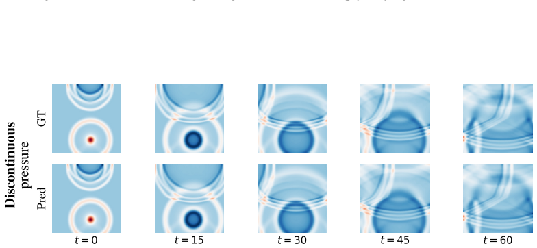
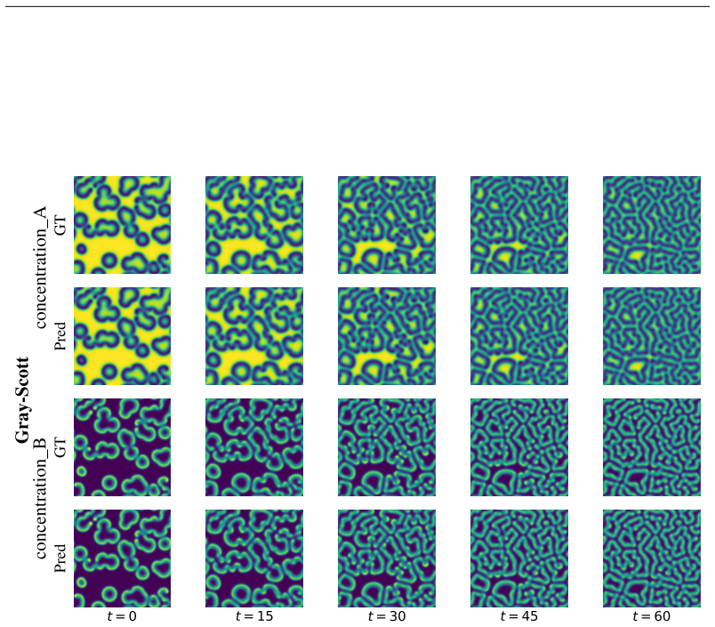
Foundation models have transformed machine learning for language and vision, but achieving comparable impact in physical simulation remains a challenge. Data heterogeneity and unstable long-term dynamics inhibit learning from sufficiently diverse dynamics, while varying resolutions and dimensionalities challenge efficient training on modern hardware. Through empirical and theoretical analysis, we incorporate new approaches to mitigate these obstacles, including a harmonic-analysis-based stabilization method, load-balanced distributed 2D and 3D training strategies, and compute-adaptive tokenization. Using these tools, we develop Walrus, a transformer-based foundation model developed primarily for fluid-like continuum dynamics. Walrus is pretrained on nineteen diverse scenarios spanning astrophysics, geoscience, rheology, plasma physics, acoustics, and classical fluids. Experiments show that Walrus outperforms prior foundation models on both short and long term prediction horizons on downstream tasks and across the breadth of pretraining data, while ablation studies confirm the value of our contributions to forecast stability, training throughput, and transfer performance over conventional approaches. Code and weights are released for community use.
Figures





Forward citations
Cited by 18 Pith papers
-
Function graph transformers universally approximate operators between function spaces
Function graph transformers use graph measures to provide a measure-theoretic framework where standard transformer components universally approximate operators between function spaces while preserving single-valued fu...
-
Breakeven complexity: A new perspective on neural partial differential equation solvers
Breakeven complexity is introduced to evaluate neural PDE solvers by total end-to-end cost, with results indicating they become advantageous for harder problems such as higher dimensions, longer rollouts, and higher R...
-
Discovering Physical Directions in Weight Space: Composing Neural PDE Experts
Fine-tuning neural PDE operators to regime endpoints reveals a physical direction in weight space that CCM uses to compose accurate merged models for new or extrapolated regimes from metadata or short prefixes.
-
Flowers: A Warp Drive for Neural PDE Solvers
Flowers, a neural PDE solver built from multihead warps alone, beats same-size Fourier/convolution/attention baselines on most tested flow and wave benchmarks.
-
OmniMol: Transferring Particle Physics Knowledge to Molecular Dynamics with Point-Edge Transformers
OmniMol transfers a billion-jet pre-trained PET foundation model from HEP to molecular dynamics via an interaction-matrix attention bias, delivering strong performance on the oMol dataset with minimal fine-tuning and ...
-
NEXUS: Neural Energy Fields for Physically Consistent Contact-Rich 3D Object Dynamics
NEXUS introduces a graph-based neural energy-field model that derives forces from scalar energy and dissipation terms to achieve physically consistent contact-rich 3D dynamics.
-
Small Models, Strong Priors: Architectural Inductive Bias for Parameter-Efficient Neural PDE Solvers
WaveLiT combines wavelet tokenization, linear attention, and multiscale pyramids to produce parameter-efficient neural PDE solvers that match much larger models on TheWell benchmarks.
-
AOT-POT: Adaptive Operator Transformation for Large-Scale PDE Pre-training
AOT-POT adaptively reshapes complex PDE solution operators via input-dependent transformations and parallel stream mixing to enable effective large-scale pre-training, yielding SOTA results on 12 benchmarks with minim...
-
Autoregressive One-Step Generative Modeling for Dynamical System Forecasting
MeLISA delivers one-step blockwise generative forecasting for dynamical systems that improves short-term accuracy and long-horizon statistical fidelity over neural operators while matching or exceeding their inference speed.
-
Autoregressive One-Step Generative Modeling for Dynamical System Forecasting
MeLISA extends pixel-space MeanFlow to one-step window-conditioned autoregressive forecasting, improving long-horizon turbulence statistics over neural-operator baselines.
-
Transformers for dynamical systems learn transfer operators in-context
Small transformers learn to forecast unseen dynamical systems in-context by using delay embeddings to recover the manifold and forecasting its invariant sets via a transfer-operator strategy.
-
Structure-Preserving Learning Improves Geometry Generalization in Neural PDEs
A geometry-conditioned Whitney-form neural network that solves a learned discrete conservation law improves out-of-distribution geometry generalization for steady-state PDEs compared with regression-based neural operators.
-
Otter Weather: Skillful and Computationally Efficient Medium-Range Weather Forecasting
Otter Weather is a spatiotemporal model that outperforms NWP baselines by 9.6% at 24h lead with under 3.5 A100-days training and extends efficiency gains to probabilistic forecasting via CRPS.
-
Sparse probes and murky physics: a case study of interpretability challenges in a foundation model for continuum dynamics
Case study applies SAE probing with enstrophy triage to a continuum-dynamics foundation model and reports intermittent feature consistency that does not align with standard physics while linking some output discrepanc...
-
jNO: A JAX Library for Neural Operator and Foundation Model Training
jNO introduces a unified JAX tracing system for data-driven and physics-informed neural operator training that compiles domains, residuals, losses, and diagnostics into one pipeline.
-
Replay-Based Continual Learning for Physics-Informed Neural Operators
A replay-based continual learning strategy for physics-informed neural operators mitigates catastrophic forgetting on prior physical problems while enabling efficient adaptation to new data using only physical constraints.
-
Foundation Models for Astrophysics
Astronomical 'foundation models' largely reuse transformers and self-supervised pretraining, but evidence of transfer to new instruments, populations, or tasks remains rare; the paper argues such evidence, not archite...
-
Towards a Foundation Model for the Martian Atmosphere
The paper reviews data sources, physical models, downstream applications, and AI techniques to outline considerations for building a foundation model for the Martian atmosphere.
Reference graph
Works this paper leans on
-
[1]
This was an artifact of merging several implementations rather than an intentional decision
Encoder and processor using different activations - The encoder layers all use GELU activations (Hendrycks & Gimpel, 2016) while the processor layers use SwiGLU. This was an artifact of merging several implementations rather than an intentional decision. On small scale experiments, we saw little difference from correcting this, so it was left as is
2016
-
[2]
However, in multiple dimensions, the padding will overlap in corners resulting in additive corner handling
Additive corner handling - In the boundary padding examples, we discussed the one- dimensional case where boundary topology is denoted by appended one-hot encoded chan- nels. However, in multiple dimensions, the padding will overlap in corners resulting in additive corner handling. Changing this to a cross-product of boundary tokens was not explored. B TR...
2014
-
[3]
For non-periodic boundaries, padding is implemented with additional channels containing binary masks for each topological boundary type
Periodic - There is not truly a boundary here and the neighboring points are on the opposite side of the domain. For non-periodic boundaries, padding is implemented with additional channels containing binary masks for each topological boundary type. Open and closed boudnaries are processed as separate channels so that the model can learn to treat each dif...
2021
-
[4]
The model is forced to learn to infer the time step from history
Variable time-stride: We sample trajectories spaced by varying ∆t where this ranges from 1 to 5 simulation steps. The model is forced to learn to infer the time step from history. This information is not provided explicitly
-
[5]
time-conditioning
Tensor-aware rotations: For all data defined on Euclidean domains, we perform additional augmentation using rotations sampled from the axis-aligned subset of SO(3). As mentioned in the main text, all geometric transformations are performed both on the spatial layout and on tensor-valued fields to ensure physical consistency. For non-Walrus models in exper...
2001
-
[6]
Pretraining data (Table 5) - Data used during pretrainingWalrus
-
[7]
C.1 DATA TRANSFORMATIONS The following elementwise transformations were applied to input fields independent of normalization
Downstream tasks (Table 6) - Data used for finetuning task which had never been seen by Walrus during initial pretraining, though Conditioned Incompressible NS from PDEArena was used during DPOT training and CE-RM from PDEGym was part of the same data collection as Poseidon’s pretraining. C.1 DATA TRANSFORMATIONS The following elementwise transformations ...
-
[9]
•turbulence gravity cooling
temperature: log10 - reduce long tail of strictly positive field in accordance with domain conventions. •turbulence gravity cooling
-
[11]
•turbulent radiative layer 3D
temperature: log10 - reduce long tail of strictly positive field in accordance with domain conventions. •turbulent radiative layer 3D
-
[12]
density: log10 - reduce long tail of strictly positive field in accordance with domain conventions
-
[13]
C.2 BOUNDARYHANDLING In the case of periodic boundary conditions, the computations described in Section 3.2 can be performed exactly
temperature: log10 - reduce long tail of strictly positive field in accordance with domain conventions. C.2 BOUNDARYHANDLING In the case of periodic boundary conditions, the computations described in Section 3.2 can be performed exactly. As Walrus is intended to be general-purpose and not constrained to settings where the boundary conditions are exactly k...
-
[14]
We do not know what is beyond the boundary
Open - The domain extends beyond the sub-domain we are currently viewing. We do not know what is beyond the boundary
-
[15]
The model is unaware of what conditions are enforced at this barrier
Closed - There is some form of barrier marking this as the limit of the domain. The model is unaware of what conditions are enforced at this barrier. 29
-
[17]
though the impact of this is not explored in this work. D MODES OFOPERATION FORDYNAMICSMODELS Ground Truth Walrus Poseidon Walrus Error Poseidon Error 0.0 0.2 0.4 0.6 0.8 1.0 0.0 0.2 0.4 0.6 0.8 Figure 13: Comparsion between Walrus and the Poseidon-L model on linear advection of smooth initial conditions. Without history, the task becomes degenerate as it...
arXiv 2024
-
[2024]
URLhttps://arxiv.org/abs/2210.07182. Ronak Tali, Ali Rabeh, Cheng-Hau Yang, Mehdi Shadkhah, Samundra Karki, Abhisek Upadhyaya, Suriya Dhakshinamoorthy, Marjan Saadati, Soumik Sarkar, Adarsh Krishnamurthy, Chinmay Hegde, Aditya Balu, and Baskar Ganapathysubramanian. Flowbench: A large scale benchmark for flow simulation over complex geometries, 2024. URL h...
Pith/arXiv arXiv 2024
discussion (0)
Sign in with ORCID, Apple, or X to comment. Anyone can read and Pith papers without signing in.