Recognition: unknown
String-inspired Gauss-Bonnet Gravity Inflation and ACT
Pith reviewed 2026-05-10 03:35 UTC · model grok-4.3
The pith
Sixteen Gauss-Bonnet inflation models all yield the observed red tilt ns ≈ 0.97 at 60 e-folds.
A machine-rendered reading of the paper's core claim, the machinery that carries it, and where it could break.
Core claim
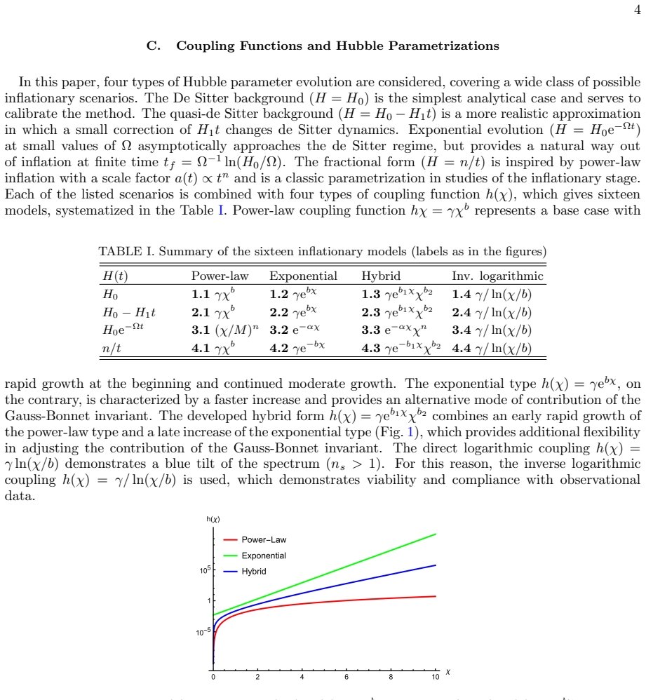
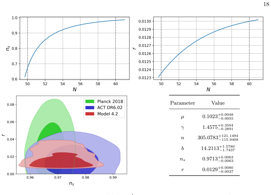
Systematic observational verification shows that all sixteen models reproduce the red spectral tilt of scalar perturbations consistent with CMB data, yielding ns ≈ 0.97 at N = 60 e-folds. The hybrid coupling h(χ) = γ e^{b1 χ} χ^{b2} interpolates between power-law and exponential forms. Dataset preference is set by the Hubble parametrization rather than the coupling function, and the parameter μ ≈ 0.1 stays stable across every configuration.
What carries the argument
The ghost-free string-inspired f(R, G) model in which the Gauss-Bonnet invariant is non-minimally coupled to an auxiliary scalar field χ through the function h(χ), together with four Hubble parametrizations and the four coupling forms (including the hybrid interpolation).
If this is right
- The stability of μ ≈ 0.1 across all models indicates it plays a fundamental role inside the ghost-free formalism.
- Hubble parametrization choice controls which dataset is preferred, allowing model selection to be guided by data type.
- The hybrid coupling supplies extra flexibility for tuning the Gauss-Bonnet contribution at different stages of inflation.
- Every combination remains viable for producing the observed red tilt of scalar perturbations.
Where Pith is reading between the lines
- Future high-precision CMB polarization data could separate the four Hubble parametrizations.
- The framework may be tested in post-inflationary epochs to check whether the same couplings remain consistent.
- The stable μ value offers a concrete target for string-theory compactification searches that seek similar effective parameters.
Load-bearing premise
The models are assumed to remain ghost-free for the chosen Hubble parametrizations and coupling functions throughout inflation.
What would settle it
A future CMB measurement that finds the scalar spectral index ns at sixty e-folds lying well outside the range near 0.97, or a clear instability in the value of μ.
Figures




read the original abstract
In this article we present a systematic observational verification of the ghost-free string-inspired $f(R,\mathcal{G})$ model, where the Gauss-Bonnet invariant is non-minimally coupled to an auxiliary scalar field $\chi$ through the coupling function $h(\chi)$. Previous studies confirmed the theoretical viability of this framework using phenomenological parameter choices. In this work, for the first time, a systematic comparison with observational data from Planck 2018 and the Atacama Comsology Telescope is carried out via a Bayesian MCMC analysis using the Cobaya code. We explore an extended set of sixteen models constructed from four types of the Hubble parameter combined with power-law, exponential, hybrid, and inverse logarithmic coupling functions $h(\chi)$. The hybrid coupling $h(\chi) = \gamma e^{b_1\chi}\chi^{b_2}$, introduced in this context, allows for interpolation between the power-law and exponential forms, providing additional flexibility in controlling the Gauss-Bonnet contribution at different stages of inflation. All sixteen models reproduce the red spectral tilt of scalar perturbations consistent with CMB observations, yielding $n_s \approx 0.97$ at $N = 60$ e-folds. We find that the preference for the dataset is systematically determined by the choice of Hubble parametrization rather than by the coupling function. The parameter $\mu\approx0.1$ remains stable in all configurations, suggesting its fundamental role within the ghost-free formalism.
Editorial analysis
A structured set of objections, weighed in public.
Referee Report
Summary. The manuscript presents a systematic Bayesian MCMC analysis using the Cobaya code of sixteen string-inspired f(R, G) gravity inflation models. These models combine four Hubble parameter parametrizations with four coupling functions h(χ) for the Gauss-Bonnet term, including a newly introduced hybrid form h(χ) = γ e^{b1 χ} χ^{b2}. The analysis compares the models to Planck 2018 and Atacama Cosmology Telescope data, claiming that all sixteen combinations yield a scalar spectral index ns ≈ 0.97 at 60 e-folds, consistent with observations, with the parameter μ ≈ 0.1 stable across all cases, and the models remaining ghost-free based on prior phenomenological studies.
Significance. If the results hold, particularly the ghost-free nature for the fitted parameters, this work offers the first detailed observational confrontation of this class of models with recent CMB data. The stability of μ and the viability of the hybrid coupling are notable strengths, as is the systematic exploration of multiple Hubble and coupling combinations. The use of standard MCMC tools adds reproducibility to the parameter constraints.
major comments (2)
- [Abstract and Results section] The claim that all sixteen models are observationally viable and ghost-free relies on the no-ghost conditions (positive kinetic coefficients for scalar and tensor modes) holding for the MCMC best-fit values of μ, γ, b1, b2. However, the manuscript invokes prior phenomenological verification without reporting an explicit re-derivation or numerical check of these conditions using the posterior means or chains from Cobaya for each of the 16 Hubble+coupling pairs. This is load-bearing for the central claim of viability.
- [MCMC analysis] The abstract reports ns ≈ 0.97 without accompanying error bars or confidence intervals from the MCMC posteriors, and no posterior plots are mentioned or described, which weakens the quantitative support for the stability of μ ≈ 0.1 across models.
minor comments (2)
- [Introduction] The hybrid coupling function is introduced as new in this context, but a brief comparison to existing literature on similar hybrid forms in other modified gravity models would enhance context.
- [Conclusion] The preference for the dataset being determined by Hubble parametrization rather than coupling function is an interesting finding; clarifying how this is quantified (e.g., via Bayes factors) would be helpful.
Simulated Author's Rebuttal
We thank the referee for the thorough review and valuable suggestions. We address each major comment below and will make the necessary revisions to enhance the manuscript's clarity and rigor.
read point-by-point responses
-
Referee: [Abstract and Results section] The claim that all sixteen models are observationally viable and ghost-free relies on the no-ghost conditions (positive kinetic coefficients for scalar and tensor modes) holding for the MCMC best-fit values of μ, γ, b1, b2. However, the manuscript invokes prior phenomenological verification without reporting an explicit re-derivation or numerical check of these conditions using the posterior means or chains from Cobaya for each of the 16 Hubble+coupling pairs. This is load-bearing for the central claim of viability.
Authors: We agree with the referee that explicitly verifying the no-ghost conditions at the MCMC-derived parameter values would provide stronger support for the viability claim. Although our previous phenomenological studies established the conditions for a range of parameters including μ ≈ 0.1, we will revise the manuscript to include a dedicated numerical check. Specifically, we will compute the kinetic coefficients for scalar and tensor modes using the best-fit values from the Cobaya chains for each of the 16 models and confirm they remain positive, reporting the results in a new table or appendix. revision: yes
-
Referee: [MCMC analysis] The abstract reports ns ≈ 0.97 without accompanying error bars or confidence intervals from the MCMC posteriors, and no posterior plots are mentioned or described, which weakens the quantitative support for the stability of μ ≈ 0.1 across models.
Authors: We acknowledge that the abstract's presentation of ns ≈ 0.97 lacks the associated uncertainties from the MCMC analysis. In the revised version, we will update the abstract to report ns with its 1σ confidence interval derived from the posterior distributions. Furthermore, we will include a description of the posterior plots in the results section and ensure that figures showing the marginalized posteriors for μ and other parameters across the models are referenced, thereby better demonstrating the stability of μ ≈ 0.1. revision: yes
Circularity Check
No significant circularity; MCMC analysis yields independent empirical results
full rationale
The paper performs a Bayesian MCMC analysis via Cobaya on sixteen combinations of Hubble parametrizations and coupling functions (including a new hybrid form) to constrain parameters against Planck 2018 and ACT data. It reports that all models can be fitted to produce ns ≈ 0.97 at N=60 with μ ≈ 0.1 stable. This constitutes standard parameter estimation against external observations rather than any derivation that reduces by construction to its own inputs. The ghost-free property is referenced to prior studies but is not claimed to be re-derived here; the current work focuses on observational viability under that maintained assumption. No self-definitional loops, fitted quantities renamed as predictions, or load-bearing self-citations appear in the derivation chain. The reported outcomes remain falsifiable by the CMB datasets.
Axiom & Free-Parameter Ledger
free parameters (2)
- μ
- γ, b1, b2
axioms (2)
- domain assumption The f(R,G) action with non-minimal Gauss-Bonnet coupling remains ghost-free for the chosen Hubble and coupling forms.
- domain assumption Slow-roll inflation with N = 60 e-folds is an adequate description of the early universe for these models.
Reference graph
Works this paper leans on
-
[1]
A. D. Linde, Lect. Notes Phys.738(2008) 1 [arXiv:0705.0164 [hep-th]]
work page Pith review arXiv 2008
-
[2]
Introduction to the theory of the early universe: Cosmological pertur- bations and inflationary theory,
D. S. Gorbunov and V. A. Rubakov, “Introduction to the theory of the early universe: Cosmological pertur- bations and inflationary theory,” Hackensack, USA: World Scientific (2011) 489 p
2011
-
[3]
Inflationary cosmology after planck 2013.arXiv preprint arXiv:1402.0526, 2014
A. Linde, arXiv:1402.0526 [hep-th]
-
[4]
D. H. Lyth and A. Riotto, Phys. Rept.314(1999) 1 [hep-ph/9807278]
work page Pith review arXiv 1999
- [5]
-
[6]
Capozziello, M
S. Capozziello, M. De Laurentis, Phys. Rept.509, 167 (2011); V. Faraoni and S. Capozziello, Fundam. Theor. Phys.170(2010)
2011
-
[7]
Nojiri, S.D
S. Nojiri, S.D. Odintsov, eConfC0602061, 06 (2006) [Int. J. Geom. Meth. Mod. Phys.4, 115 (2007)]
2006
-
[8]
Nojiri, S.D
S. Nojiri, S.D. Odintsov, Phys. Rept.505, 59 (2011)
2011
-
[9]
J. c. Hwang and H. Noh, Phys. Rev. D71(2005) 063536 doi:10.1103/PhysRevD.71.063536 [gr-qc/0412126]
-
[10]
S. Nojiri, S. D. Odintsov and M. Sami, Phys. Rev. D74(2006) 046004 doi:10.1103/PhysRevD.74.046004 [hep-th/0605039]
-
[11]
G. Cognola, E. Elizalde, S. Nojiri, S. Odintsov and S. Zerbini, Phys. Rev. D75(2007) 086002 doi:10.1103/PhysRevD.75.086002 [hep-th/0611198]
-
[12]
S. Nojiri, S. D. Odintsov and M. Sasaki, Phys. Rev. D71(2005) 123509 doi:10.1103/PhysRevD.71.123509 [hep-th/0504052]
-
[13]
S. Nojiri and S. D. Odintsov, Phys. Lett. B631(2005) 1 doi:10.1016/j.physletb.2005.10.010 [hep-th/0508049]. 21
-
[14]
M. Satoh, S. Kanno and J. Soda, Phys. Rev. D77(2008) 023526 doi:10.1103/PhysRevD.77.023526 [arXiv:0706.3585 [astro-ph]]
-
[15]
K. Bamba, A. N. Makarenko, A. N. Myagky and S. D. Odintsov, JCAP1504(2015) 001 doi:10.1088/1475- 7516/2015/04/001 [arXiv:1411.3852 [hep-th]]
-
[16]
Z. Yi, Y. Gong and M. Sabir, Phys. Rev. D98(2018) no.8, 083521 doi:10.1103/PhysRevD.98.083521 [arXiv:1804.09116 [gr-qc]]
-
[17]
Z. K. Guo and D. J. Schwarz, Phys. Rev. D80(2009) 063523 doi:10.1103/PhysRevD.80.063523 [arXiv:0907.0427 [hep-th]]
-
[18]
Z. K. Guo and D. J. Schwarz, Phys. Rev. D81(2010) 123520 doi:10.1103/PhysRevD.81.123520 [arXiv:1001.1897 [hep-th]]
-
[19]
P. X. Jiang, J. W. Hu and Z. K. Guo, Phys. Rev. D88(2013) 123508 doi:10.1103/PhysRevD.88.123508 [arXiv:1310.5579 [hep-th]]
-
[20]
C. van de Bruck, K. Dimopoulos, C. Longden and C. Owen, arXiv:1707.06839 [astro-ph.CO]
-
[21]
E. O. Pozdeeva, M. R. Gangopadhyay, M. Sami, A. V. Toporensky and S. Y. Vernov, Phys. Rev. D102 (2020) no.4, 043525 doi:10.1103/PhysRevD.102.043525 [arXiv:2006.08027 [gr-qc]]
-
[22]
S. Vernov and E. Pozdeeva, Universe7(2021) no.5, 149 doi:10.3390/universe7050149 [arXiv:2104.11111 [gr- qc]]
-
[23]
E. O. Pozdeeva and S. Y. Vernov, Eur. Phys. J. C81(2021) no.7, 633 doi:10.1140/epjc/s10052-021-09435-8 [arXiv:2104.04995 [gr-qc]]
-
[24]
I. Fomin, Eur. Phys. J. C80(2020) no.12, 1145 doi:10.1140/epjc/s10052-020-08718-w [arXiv:2004.08065 [gr-qc]]
-
[25]
M. De Laurentis, M. Paolella and S. Capozziello, Phys. Rev. D91(2015) no.8, 083531 doi:10.1103/PhysRevD.91.083531 [arXiv:1503.04659 [gr-qc]]
-
[26]
Scalar Field Cosmology, S. Chervon, I. Fomin, V. Yurov and A. Yurov, World Scientific 2019, doi:10.1142/11405
-
[27]
K. Nozari and N. Rashidi, Phys. Rev. D95(2017) no.12, 123518 doi:10.1103/PhysRevD.95.123518 [arXiv:1705.02617 [astro-ph.CO]]
-
[28]
S. D. Odintsov and V. K. Oikonomou, Phys. Rev. D98(2018) no.4, 044039 doi:10.1103/PhysRevD.98.044039 [arXiv:1808.05045 [gr-qc]]
-
[29]
S. Kawai, M. a. Sakagami and J. Soda, Phys. Lett. B437, 284 (1998) doi:10.1016/S0370-2693(98)00925-3 [gr-qc/9802033]
-
[30]
Z. Yi and Y. Gong, Universe5(2019) no.9, 200 doi:10.3390/universe5090200 [arXiv:1811.01625 [gr-qc]]
-
[31]
C. van de Bruck, K. Dimopoulos and C. Longden, Phys. Rev. D94(2016) no.2, 023506 doi:10.1103/PhysRevD.94.023506 [arXiv:1605.06350 [astro-ph.CO]]
-
[32]
K. i. Maeda, N. Ohta and R. Wakebe, Eur. Phys. J. C72(2012) 1949 doi:10.1140/epjc/s10052-012-1949-6 [arXiv:1111.3251 [hep-th]]
-
[33]
W. Y. Ai, Commun. Theor. Phys.72(2020) no.9, 095402 doi:10.1088/1572-9494/aba242 [arXiv:2004.02858 [gr-qc]]
-
[34]
R. Easther and K. i. Maeda, Phys. Rev. D54(1996) 7252 doi:10.1103/PhysRevD.54.7252 [hep-th/9605173]
-
[35]
A. Codello and R. K. Jain, Class. Quant. Grav.33(2016) no.22, 225006 doi:10.1088/0264-9381/33/22/225006 [arXiv:1507.06308 [gr-qc]]
-
[36]
V. K. Oikonomou, Class. Quant. Grav.38(2021) no.19, 195025 doi:10.1088/1361-6382/ac2168 [arXiv:2108.10460 [gr-qc]]
-
[37]
S. D. Odintsov, V. K. Oikonomou and F. P. Fronimos, Nucl. Phys. B958(2020), 115135 doi:10.1016/j.nuclphysb.2020.115135 [arXiv:2003.13724 [gr-qc]]
-
[38]
V. K. Oikonomou, Phys. Lett. B856(2024), 138890 doi:10.1016/j.physletb.2024.138890 [arXiv:2407.12155 [gr-qc]]
- [39]
-
[40]
V. K. Oikonomou, P. D. Katzanis and I. C. Papadimitriou, Class. Quant. Grav.39(2022) no.9, 095008 doi:10.1088/1361-6382/ac5eba [arXiv:2203.09867 [gr-qc]]
-
[41]
V. K. Oikonomou, Astropart. Phys.141(2022), 102718 doi:10.1016/j.astropartphys.2022.102718 [arXiv:2204.06304 [gr-qc]]
-
[42]
S. Nojiri, S. D. Odintsov, V. K. Oikonomou and A. A. Popov, Nucl. Phys. B973(2021), 115617 doi:10.1016/j.nuclphysb.2021.115617 [arXiv:2111.09457 [gr-qc]]
-
[43]
S. Nojiri, S. D. Odintsov, V. K. Oikonomou, N. Chatzarakis and T. Paul, Eur. Phys. J. C79(2019) no.7, 565 doi:10.1140/epjc/s10052-019-7080-1 [arXiv:1907.00403 [gr-qc]]
-
[44]
Planck 2018 results. X. Constraints on inflation
Y. Akramiet al.[Planck], Astron. Astrophys.641(2020), A10 doi:10.1051/0004-6361/201833887 [arXiv:1807.06211 [astro-ph.CO]]
work page internal anchor Pith review doi:10.1051/0004-6361/201833887 2020
-
[45]
P. A. R. Adeet al.[BICEP and Keck], Phys. Rev. Lett.127(2021) no.15, 151301 doi:10.1103/PhysRevLett.127.151301 [arXiv:2110.00483 [astro-ph.CO]]
-
[46]
The Atacama Cosmology Telescope: DR6 Power Spectra, Likelihoods and $\Lambda$CDM Parameters
T. Louiset al.[ACT], [arXiv:2503.14452 [astro-ph.CO]]
work page internal anchor Pith review arXiv
- [47]
- [48]
- [49]
-
[50]
L. Liu, Z. Yi and Y. Gong, [arXiv:2505.02407 [astro-ph.CO]]
work page internal anchor Pith review Pith/arXiv arXiv
-
[51]
Yogesh, A. Mohammadi, Q. Wu and T. Zhu, [arXiv:2505.05363 [astro-ph.CO]]
- [52]
- [53]
- [54]
- [55]
- [56]
- [57]
- [58]
- [59]
- [60]
-
[61]
A. Mohammadi, Yogesh and A. Wang, [arXiv:2507.06544 [astro-ph.CO]]
-
[62]
What new physics can we extract from inflation using the
S. Choudhury, G. Bauyrzhan, S. K. Singh and K. Yerzhanov, [arXiv:2506.15407 [astro-ph.CO]]
-
[63]
S. D. Odintsov and V. K. Oikonomou, Phys. Lett. B868(2025), 139779 doi:10.1016/j.physletb.2025.139779 [arXiv:2506.08193 [gr-qc]]
- [64]
- [65]
-
[66]
G. Kouniatalis and E. N. Saridakis, [arXiv:2507.17721 [astro-ph.CO]]
- [67]
-
[68]
C. Dioguardi, A. J. Iovino and A. Racioppi, Phys. Lett. B868(2025), 139664 doi:10.1016/j.physletb.2025.139664 [arXiv:2504.02809 [gr-qc]]
-
[69]
J. Yuennan, P. Koad, F. Atamurotov and P. Channuie, [arXiv:2508.17263 [astro-ph.CO]]
- [70]
-
[71]
H. J. Kuralkar, S. Panda and A. Vidyarthi, JCAP05(2025), 073 doi:10.1088/1475-7516/2025/05/073 [arXiv:2502.03573 [astro-ph.CO]]
- [72]
- [73]
- [74]
- [75]
-
[76]
Inflation with Gauss-Bonnet Correction and Higgs Potential
Z. Ahghari and M. Farhoudi, [arXiv:2512.12286 [gr-qc]]
work page internal anchor Pith review Pith/arXiv arXiv
-
[77]
E. McDonough and E. G. M. Ferreira, [arXiv:2512.05108 [astro-ph.CO]]
-
[78]
D. Chakraborty, M. Hai, S. T. Jahan, A. R. Kamal and M. S. J. Shuvo, [arXiv:2511.19610 [hep-th]]
-
[79]
S. Noori Gashti, M. A. S. Afshar, M. R. Alipour, B. Pourhassan and J. Sadeghi, Eur. Phys. J. C85(2025) no.11, 1343 doi:10.1140/epjc/s10052-025-15066-0
-
[80]
J. Yuennan, F. Atamurotov and P. Channuie, [arXiv:2511.17216 [astro-ph.CO]]
discussion (0)
Sign in with ORCID, Apple, or X to comment. Anyone can read and Pith papers without signing in.