Recognition: 3 theorem links
· Lean TheoremAnalytic Bridge Diffusions for Controlled Path Generation
Pith reviewed 2026-05-08 19:23 UTC · model grok-4.3
The pith
Linear-quadratic-Gaussian control with Gaussian-mixture boundaries supplies closed-form scores, marginals, and protocols for bridge diffusions.
A machine-rendered reading of the paper's core claim, the machinery that carries it, and where it could break.
Core claim
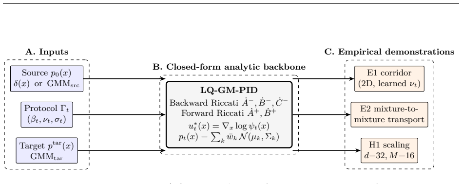
Recasting the classical linear-quadratic-Gaussian stochastic-control problem as a path-integral diffusion task with Gaussian-mixture initial and terminal laws keeps the Riccati equations closed-form. Consequently the score function, the time-dependent marginal densities, and the optimal control protocol are all available by direct matrix operations rather than by simulation or neural approximation.
What carries the argument
LQ-GM-PID: the linear-quadratic-Gaussian path-integral diffusion that replaces point-terminal regulation by a prescribed Gaussian-mixture density while preserving Riccati solvability.
If this is right
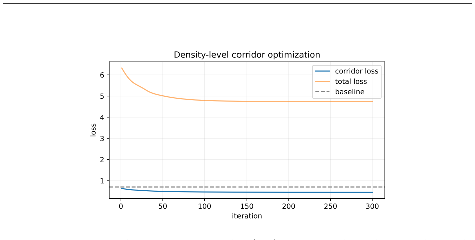
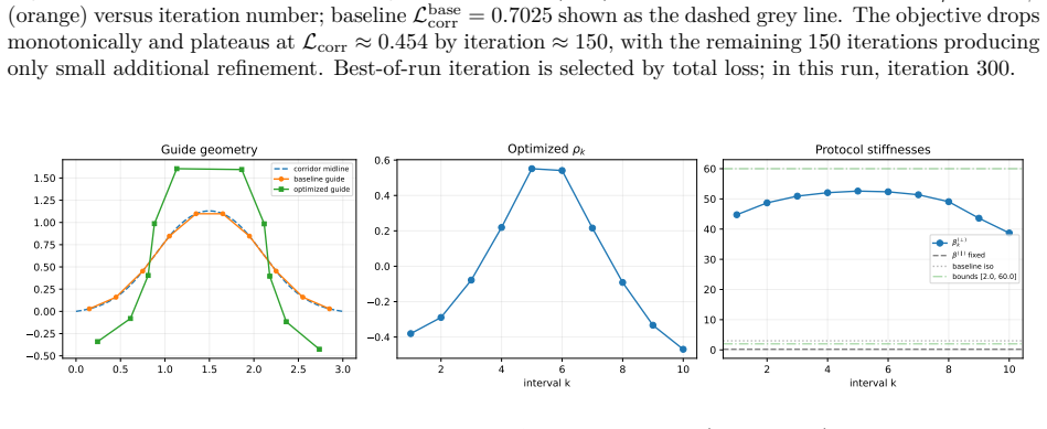
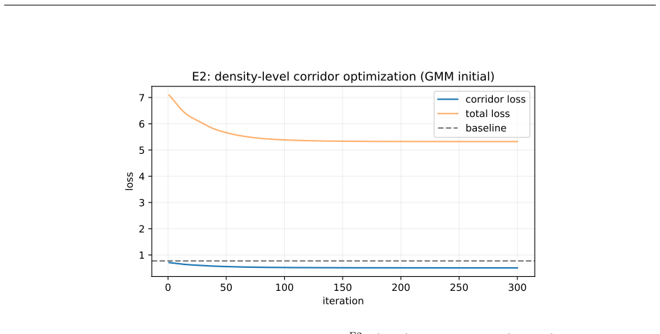
- Exact path shaping is demonstrated on a 2D corridor task and a 2D multi-entrance transport task.
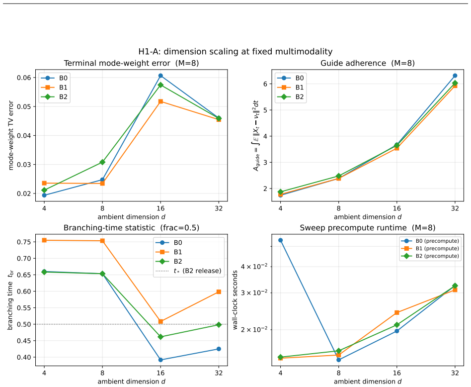
- The same analytic pipeline scales to dimension 32 with 16 Gaussian-mixture modes using sub-50 ms precompute on a laptop.
- Bridge diffusion becomes a tool for explicit path shaping rather than terminal matching alone.
- The construction supplies an exact benchmark against which neural score estimates and protocol-learning procedures can be validated.
Where Pith is reading between the lines
- The closed-form gradients may be used to initialize or regularize neural bridge models on nearby non-Gaussian problems.
- The same Riccati structure could be reused to derive analytic reference trajectories for sampling or planning algorithms outside diffusion models.
- Because intermediate marginals are explicit, the method offers a direct testbed for studying how control objectives affect sample diversity at every time slice.
Load-bearing premise
Linear dynamics, Gaussian noise, quadratic costs, and Gaussian-mixture boundary laws together suffice to keep the Riccati solution closed-form when the terminal target is a full density instead of a single point.
What would settle it
A numerical check in which the analytic score or marginal density for a chosen Gaussian-mixture terminal differs from the histogram obtained by direct forward simulation of the controlled linear diffusion.
Figures


read the original abstract
Most modern bridge-diffusion methods achieve finite-time transport by specifying an interpolation, Schr\"odinger-bridge, or stochastic-control objective and then learning the associated score or drift field with a neural network. In contrast, we identify a restricted but sufficiently broad and analytically solvable class in which the score, intermediate marginals, and protocol gradients are available in closed form without inner stochastic simulation loops and without neural networks in the optimization loop. We recast the classical linear--quadratic--Gaussian (LQG) stochastic-control structure as a transport problem of the Path Integral Diffusion (PID) type. In classical LQG control, linear dynamics, Gaussian noise, and quadratic costs lead to Riccati equations and closed-form optimal feedback. In LQ-GM-PID, we retain the linear--quadratic stochastic-control backbone, but replace terminal state regulation by a prescribed terminal probability density and allow both the initial and terminal laws to be Gaussian Mixtures (GM). Moreover, LQ-GM-PID turns bridge diffusion from a tool for terminal target matching alone into a tool for path shaping. We demonstrate this on a 2D corridor task, a 2D multi-entrance transport task, and a high-dimensional scaling study with $d=32$ and $M=16$ Gaussian-mixture terminal modes, all with sub-50\,ms analytic precompute on a laptop. We position LQ-GM-PID as an analytically solvable reference model for the state-of-the-art neural bridge-diffusion and generative-transport methods: a controlled setting in which neural approximations, score estimates, path-shaping objectives, and protocol-learning procedures can be tested against exact quantities.
Editorial analysis
A structured set of objections, weighed in public.
Referee Report
Summary. The paper proposes LQ-GM-PID, an analytically solvable bridge-diffusion framework obtained by recasting classical linear-quadratic-Gaussian (LQG) stochastic control as a path-integral-diffusion transport problem. Linear dynamics, quadratic costs, and Gaussian-mixture initial/terminal laws are retained so that the score function, intermediate marginals, and protocol gradients remain available in closed form via Riccati equations, without neural networks or inner stochastic simulation loops. The method is demonstrated on 2-D corridor and multi-entrance tasks plus a d=32, M=16 scaling study, and is positioned as an exact reference model against which neural bridge-diffusion and generative-transport algorithms can be benchmarked.
Significance. If the closed-form claims hold, the work supplies a computationally cheap (sub-50 ms pre-compute) and fully reproducible reference class for controlled path generation. It converts bridge diffusion from a terminal-matching tool into an explicit path-shaping instrument while preserving the classical LQG solvability structure, thereby offering a concrete test-bed for score estimation, path-shaping objectives, and protocol-learning procedures in the neural literature.
major comments (2)
- [Abstract / LQ-GM-PID section] Abstract and LQ-GM-PID formulation: the central claim that replacing the terminal point target by a prescribed Gaussian-mixture density nevertheless keeps the Riccati solution closed-form (and therefore yields analytic scores, marginals, and gradients) is asserted without an explicit derivation or propagation argument. Standard LQG Riccati theory assumes a quadratic terminal cost centered at a fixed point; the paper must show how the mixture structure is propagated through the HJB or Riccati equation without introducing mode-selection approximations or numerical solves.
- [Abstract] Abstract: the statement that “the score, intermediate marginals, and protocol gradients are available in closed form without inner stochastic simulation loops” is load-bearing for the entire contribution, yet the provided text supplies neither the explicit Riccati expressions for the GM case nor an error analysis confirming that analyticity is preserved for all claimed quantities.
Simulated Author's Rebuttal
We thank the referee for the careful reading and for identifying the need for a more explicit derivation of the closed-form properties. We agree these details are central and will revise the manuscript to include them.
read point-by-point responses
-
Referee: [Abstract / LQ-GM-PID section] Abstract and LQ-GM-PID formulation: the central claim that replacing the terminal point target by a prescribed Gaussian-mixture density nevertheless keeps the Riccati solution closed-form (and therefore yields analytic scores, marginals, and gradients) is asserted without an explicit derivation or propagation argument. Standard LQG Riccati theory assumes a quadratic terminal cost centered at a fixed point; the paper must show how the mixture structure is propagated through the HJB or Riccati equation without introducing mode-selection approximations or numerical solves.
Authors: We agree that the manuscript asserts the closed-form property at a high level without a full propagation argument. In the revision we will add a dedicated derivation subsection. Because the dynamics remain linear, each terminal Gaussian component admits an independent Riccati solution for its quadratic cost centered at its own mean. The intermediate marginals are then exactly the corresponding mixture of Gaussians propagated forward under the linear dynamics (mixture weights unchanged). The score is the gradient of the log of this mixture density, which is an explicit weighted sum of the per-component scores and therefore analytic. Protocol gradients follow by direct differentiation of the same expression. No mode-selection or numerical solves are introduced; the mixture is retained at every time step. revision: yes
-
Referee: [Abstract] Abstract: the statement that “the score, intermediate marginals, and protocol gradients are available in closed form without inner stochastic simulation loops” is load-bearing for the entire contribution, yet the provided text supplies neither the explicit Riccati expressions for the GM case nor an error analysis confirming that analyticity is preserved for all claimed quantities.
Authors: We concur that explicit Riccati expressions and an analyticity confirmation are required. The revised manuscript will present the per-mode Riccati equations (backward propagation of the quadratic value-function coefficients for each mixture component) together with the forward evolution rules for the mixture means, covariances, and weights. Because every operation is either a linear transformation or a closed-form Gaussian integral, the resulting score, marginal densities, and gradients remain exact analytic expressions with no approximation error or inner simulation. We will also add a short error-analysis paragraph confirming that the quantities coincide with the classical LQG solutions on each component and that the mixture combination introduces no additional error. revision: yes
Circularity Check
No circularity: derivation rests on external classical LQG Riccati theory
full rationale
The paper recasts the established linear-quadratic-Gaussian stochastic control framework (with its Riccati equations and closed-form feedback) as a bridge-diffusion transport problem, extending the terminal condition to a Gaussian-mixture density while retaining the LQ backbone. This extension is presented as a direct, analytic consequence of the retained structure rather than any internal fitting, self-definition, or load-bearing self-citation. No equation or claim reduces by construction to a parameter estimated inside the paper, and the cited LQG results are classical external benchmarks independent of the present work. The derivation chain therefore remains self-contained.
Axiom & Free-Parameter Ledger
free parameters (2)
- Quadratic cost matrices Q and R
- Gaussian-mixture parameters (means, covariances, weights for initial and terminal)
axioms (2)
- standard math Linear dynamics driven by Gaussian noise under linear feedback produce Gaussian marginals at every time.
- standard math The finite-horizon Riccati equation admits a unique positive-definite solution under the usual controllability/observability conditions.
Lean theorems connected to this paper
-
Cost.FunctionalEquation (J = ½(x+x⁻¹)−1, Aczél uniqueness)washburn_uniqueness_aczel unclear?
unclearRelation between the paper passage and the cited Recognition theorem.
We retain the linear–quadratic stochastic-control backbone, but replace terminal state regulation by a prescribed terminal probability density and allow both the initial and terminal laws to be Gaussian Mixtures (GM).
-
Foundation.BranchSelection / CostRCLCombiner_isCoupling_iff unclear?
unclearRelation between the paper passage and the cited Recognition theorem.
V_t(x) = ½(x−ν_t)ᵀ β_t (x−ν_t) ... Riccati equations and closed-form optimal feedback.
What do these tags mean?
- matches
- The paper's claim is directly supported by a theorem in the formal canon.
- supports
- The theorem supports part of the paper's argument, but the paper may add assumptions or extra steps.
- extends
- The paper goes beyond the formal theorem; the theorem is a base layer rather than the whole result.
- uses
- The paper appears to rely on the theorem as machinery.
- contradicts
- The paper's claim conflicts with a theorem or certificate in the canon.
- unclear
- Pith found a possible connection, but the passage is too broad, indirect, or ambiguous to say the theorem truly supports the claim.
Reference graph
Works this paper leans on
-
[1]
arXiv:2409.08861 [cs, math, stat]
URLhttp://arxiv.org/abs/2409.08861. arXiv:2409.08861 [cs, math, stat]. Yuanqi Du, Michael Plainer, Rob Brekelmans, Chenru Duan, Frank Noé, Carla P. Gomes, Alán Aspuru- Guzik, and Kirill Neklyudov. Doob’s Lagrangian: A Sample-Efficient Variational Approach to Transition Path Sampling, December 2024. URLhttp://arxiv.org/abs/2410.07974. arXiv:2410.07974 [cs]...
-
[2]
ISSN 1072-3374, 1573-8795. doi: 10.1007/s10958-006-0049-2. URLhttp://link.springer.com/ 10.1007/s10958-006-0049-2. H. J. Kappen. Path integrals and symmetry breaking for optimal control theory.Journal of Statistical Mechanics: Theory and Experiment, pp. P11011, 2005a. Hilbert J. Kappen. Linear Theory for Control of Nonlinear Stochastic Systems.Phys. Rev. ...
-
[3]
Initialize att=εwith large values consistent with Eq. (48–49)
-
[4]
Propagate forward coefficients on each interval using §A.4, enforcing continuity
-
[5]
(B) Backward sweep
CacheA (+) T−ε,B (+) T−ε,θ(+) x;T−ε. (B) Backward sweep
-
[6]
Initialize att=T−εwith large values consistent with Eq. (46–47)
-
[7]
(C) Evaluate at timet
Propagate backward coefficients on each interval using §A.4, enforcing continuity. (C) Evaluate at timet
-
[8]
PrecomputeP k = Σ −1 k
-
[9]
FormS k,t =C (−) t +P k−A(+) T−ε andq k,t =θ(−) y;t +P kmk−B(+) T−εx0−θ(+) x;T−ε
-
[10]
(89–90) (use linear solves)
ComputeΛ k,t andλk,t via Eq. (89–90) (use linear solves)
-
[11]
Compute responsibilities by log-sum-exp fromlogψk,t(x)in Eq. (88)
-
[12]
unit protocol
Outputu ∗ t (x) =κt ∑ kρk,t(x)(−Λk,tx+λk,t); optionally computep∗ t (x). 31 A.6 From Gaussian-Mixture to Gaussian-Mixture: Coordinate-Shift Construction In §A.5 we assumed a deterministic startp(0) =δ(·−x0). We now extend the construction to aGaussian- Mixture initial distribution p(in)(x) = M0∑ i=1 w(0) i N(x;m (0) i ,Σ (0) i ), w (0) i >0, ∑ i w(0) i = ...
-
[13]
For each particlen= 1,...,B: drawz (n)∼p(in) and set˜x(n) 0 = 0
-
[14]
(b) Computez-independent quantities:S k,Λ k,B (−)S−1 k
For each timestepi= 0,...,N−1: (a) Evaluate the base backward coefficients and shift-propagator matrices atti. (b) Computez-independent quantities:S k,Λ k,B (−)S−1 k . (c) For each particle: applyz-corrections Eq. (111–113) and evaluate˜u∗ t (˜x(n) t ;z (n))via Eq. (114). (d) Euler–Maruyama:˜x(n) ti+1 = ˜x(n) ti + ˜u∗∆t+ √ κ∆tξ(n)
-
[15]
product-coupling
Return physical trajectoriesx(n) t = ˜x(n) t +z (n). Remark (exact vs. approximate).The coordinate-shift construction isexactfor each realisation of z: the shifted problem(˜νk,˜mj,˜x0 = 0)is a standard LQ-GM-PID instance with a deterministic start, for which all the closed-form machinery of §A.4–A.5 applies without approximation. The only discretisation e...
discussion (0)
Sign in with ORCID, Apple, or X to comment. Anyone can read and Pith papers without signing in.