Photometry is all you need: supernova classification as a mixing problem
Pith reviewed 2026-06-29 09:29 UTC · model grok-4.3
The pith
Supernovae Ia and Ibc can be classified with at least 90 percent accuracy from photometry alone by optimizing the mixing fraction in a Gaussian mixture model on light-curve fit parameters.
A machine-rendered reading of the paper's core claim, the machinery that carries it, and where it could break.
Core claim
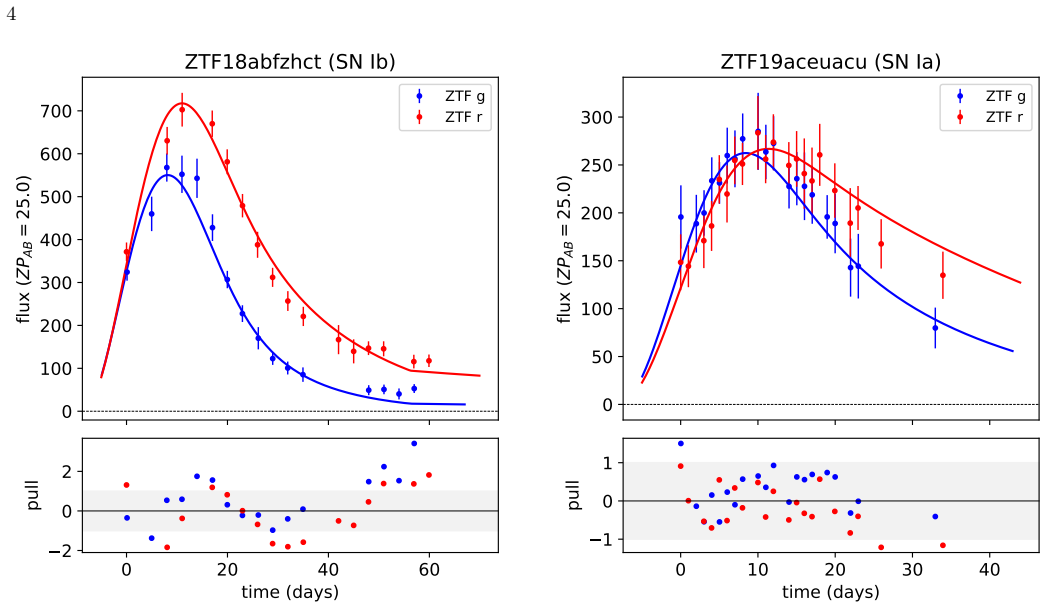
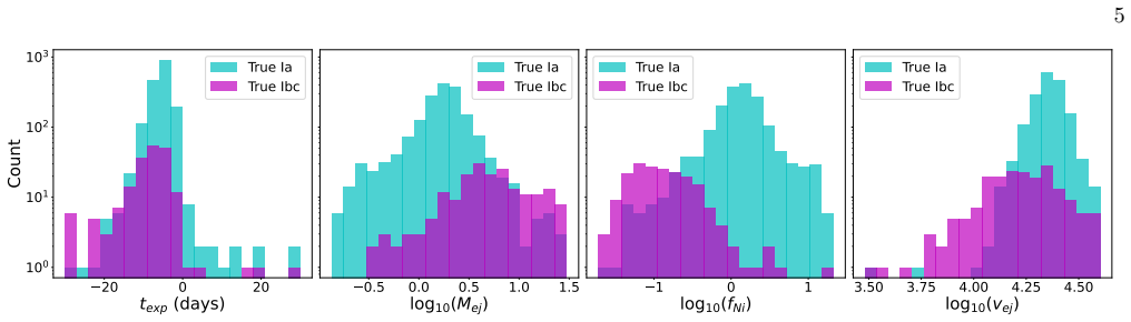
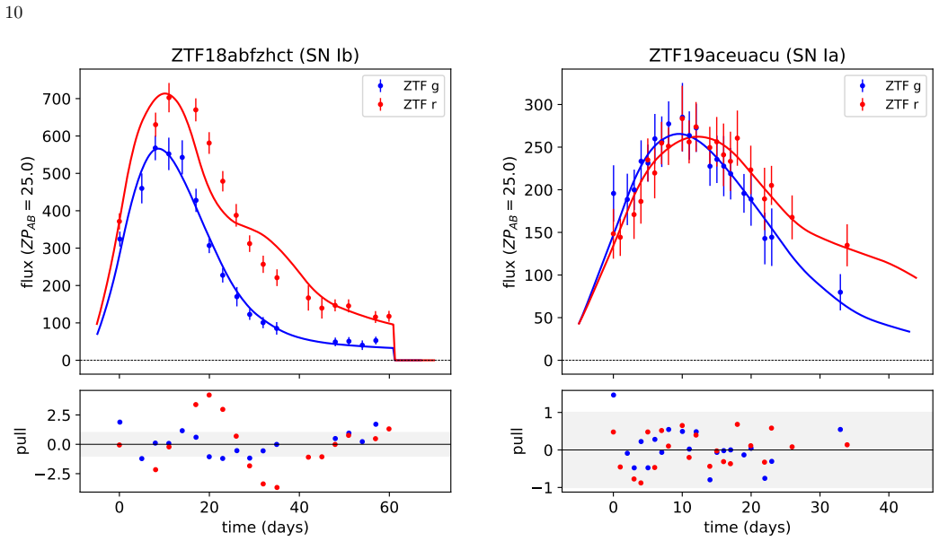
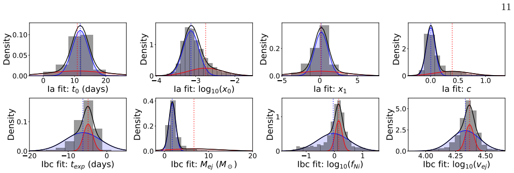
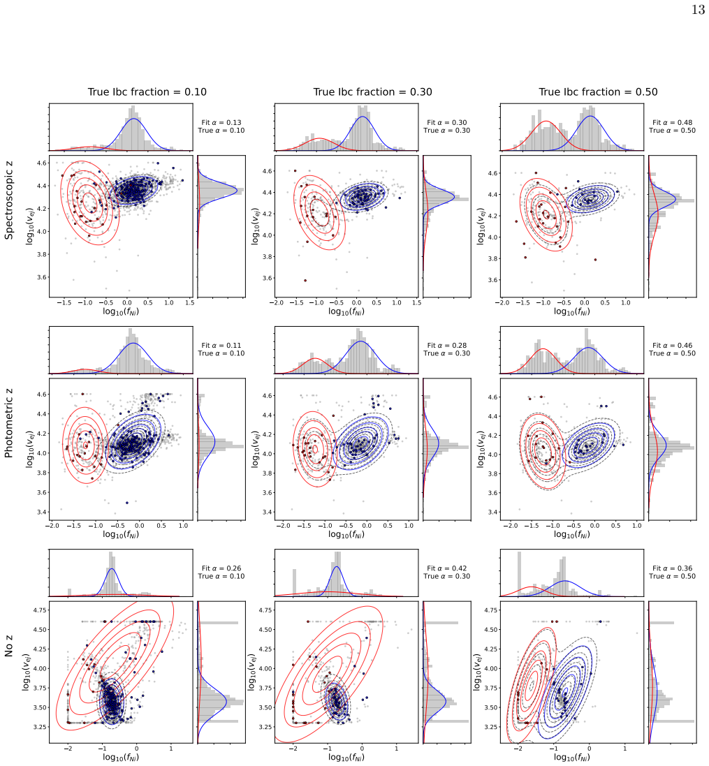
Fitting all supernova light curves with a semi-analytical model powered by radioactive decay produces distributions of fit parameters that are adequately described by a two-component Gaussian mixture model; optimizing the shared mixing fraction between the Ia and Ibc populations from the photometry alone recovers the population ratio and classifies individual events with at least 90 percent accuracy without any labeled spectroscopic dataset.
What carries the argument
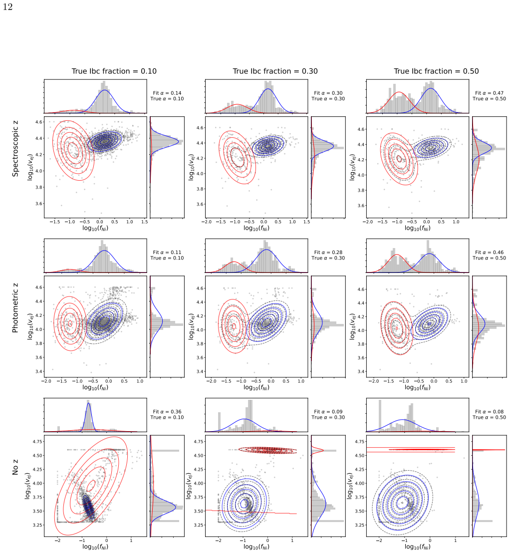
Two-component Gaussian mixture model on the distributions of fit parameters obtained from the semi-analytical radioactive-decay light-curve model, with the mixing fraction optimized to match the observed population.
If this is right
- The ratio of Ia to Ibc populations can be reliably constrained from photometry across a range of mixing fractions.
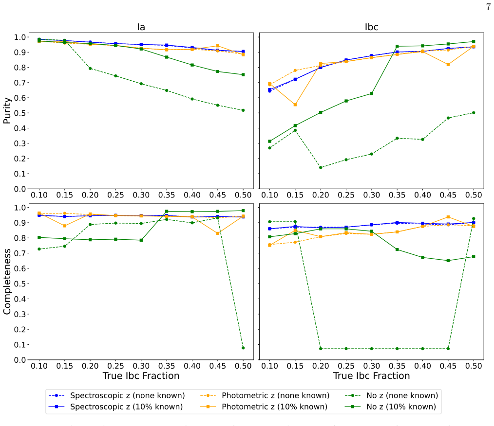
- Classification performance holds when redshift information is included, excluded, or replaced by photometric redshifts.
- A small number of known labels can be incorporated without changing the core unsupervised procedure.
- The method remains viable for fast population characterization in large photometric datasets.
Where Pith is reading between the lines
- The same mixing-model strategy could be applied to other transient classes if suitable physical light-curve models exist for them.
- Reliance on spectroscopic follow-up for classification could be substantially reduced in upcoming wide-field surveys.
- Physical model fitting may serve as a general substitute for hand-crafted features in other unsupervised astronomical classification problems.
Load-bearing premise
The fit-parameter distributions produced by the semi-analytical model for Ia and Ibc events are adequately described by a two-component Gaussian mixture whose shared mixing fraction can be optimized from photometry alone.
What would settle it
A test set of spectroscopically confirmed supernovae where the parameter distributions deviate strongly from two Gaussians or where the optimized mixing fraction yields classification accuracy well below 90 percent when compared to the true labels.
Figures
read the original abstract
In the era of large-scale photometric surveys, scalable and robust methods for classifying supernova (SN) populations are increasingly necessary. Often, spectroscopy is essential in addition to photometry to reliably classify SNe; however, complete spectroscopic follow-up is infeasible for all of the millions of transient light curves being collected by facilities such as the Vera C. Rubin Observatory. Using light curves of SNe Ia and Ibc observed with the Zwicky Transient Facility, we frame the classification of large SN populations as a mixing problem. We fit all objects using a semi-analytical SN model powered by radioactive decay, and we model the resulting distributions of fit parameters with a Gaussian Mixture model to optimize the shared population mixing fraction. This approach allows us to reliably constrain the ratio of the populations and classify SNe Ia and Ibc with $\geq$ 90% accuracy without any need for labeled training data, i.e., a spectroscopic dataset. We validate this method for varying population mixing fractions and explore the impact of including spectroscopic, photometric, or no redshift information, and a small amount of known labels. Overall, this method allows for fast and accurate SN classification and population characterization using only photometry.
Editorial analysis
A structured set of objections, weighed in public.
Referee Report
Summary. The manuscript frames supernova classification as an unsupervised mixing problem: light curves from ZTF are fit with a semi-analytical radioactive-decay model; the resulting parameter vectors are modeled as a two-component Gaussian mixture whose shared mixing fraction is optimized by maximum likelihood on the unlabeled photometry alone; the fitted fraction then yields per-object Ia/Ibc classifications claimed to reach ≥90% accuracy without spectroscopic labels. The approach is tested for varying mixing fractions and with/without redshift information.
Significance. If the GMM assumption on the fit-parameter distributions holds and the accuracy claim is quantitatively substantiated, the method would provide a scalable, label-free route to both population-ratio estimation and individual classification for the millions of transients expected from Rubin Observatory, reducing dependence on scarce spectroscopic resources.
major comments (2)
- [Abstract] Abstract: the central claim of ≥90% classification accuracy on ZTF data across mixing fractions is stated without any quantitative validation metrics, confusion matrices, error budgets, or tests against model misspecification; this leaves the performance assertion unsupported by evidence visible in the manuscript.
- [Methods (GMM fitting)] The weakest assumption (semi-analytical model produces parameter vectors whose Ia and Ibc marginals are each adequately described by a single Gaussian, with components sufficiently separated that a shared mixing fraction can be recovered by ML fitting to unlabeled data) is load-bearing for both the mixing-fraction recovery and the subsequent classification accuracy; no explicit check that the actual ZTF-derived distributions satisfy this (e.g., via skewness, multimodality, or overlap diagnostics) is provided.
minor comments (1)
- [Methods] Notation for the semi-analytical model parameters and the GMM covariance structure should be defined once in a dedicated subsection rather than introduced piecemeal.
Simulated Author's Rebuttal
We thank the referee for their constructive and detailed comments, which help clarify the presentation of our results. We respond to each major comment below.
read point-by-point responses
-
Referee: [Abstract] Abstract: the central claim of ≥90% classification accuracy on ZTF data across mixing fractions is stated without any quantitative validation metrics, confusion matrices, error budgets, or tests against model misspecification; this leaves the performance assertion unsupported by evidence visible in the manuscript.
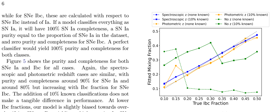
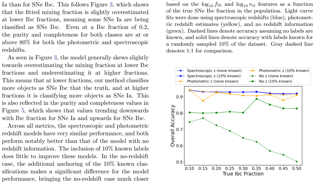
Authors: The quantitative validation, including accuracy as a function of mixing fraction, confusion matrices, and performance with/without redshift, appears in Section 4 and the associated figures. To ensure the abstract claim is immediately supported by visible evidence, we will revise the abstract to include a concise reference to the validation metrics and results. revision: yes
-
Referee: [Methods (GMM fitting)] The weakest assumption (semi-analytical model produces parameter vectors whose Ia and Ibc marginals are each adequately described by a single Gaussian, with components sufficiently separated that a shared mixing fraction can be recovered by ML fitting to unlabeled data) is load-bearing for both the mixing-fraction recovery and the subsequent classification accuracy; no explicit check that the actual ZTF-derived distributions satisfy this (e.g., via skewness, multimodality, or overlap diagnostics) is provided.
Authors: We agree that explicit diagnostics would strengthen the manuscript. In revision we will add a dedicated subsection (or appendix) containing skewness, multimodality, and overlap diagnostics on the ZTF-derived parameter distributions, together with Q-Q plots and component-separation metrics, to directly substantiate the single-Gaussian assumption per class. revision: yes
Circularity Check
No circularity; unsupervised GMM inference on model-fit parameters is independent of target labels
full rationale
The paper fits a semi-analytical radioactive-decay model to photometric light curves, extracts parameter vectors, and optimizes a shared mixing fraction via maximum-likelihood GMM on the unlabeled distribution. This procedure uses only the photometry-derived parameters and does not reduce to a fit of the target labels or a self-referential definition. Validation against known labels occurs after inference and does not enter the mixing-fraction optimization. No self-citation chains, uniqueness theorems, or ansatzes smuggled via prior work are invoked in the derivation. The GMM Gaussianity assumption is an explicit modeling choice whose validity can be tested externally rather than a definitional loop.
Axiom & Free-Parameter Ledger
free parameters (2)
- population mixing fraction
- semi-analytical model parameters
axioms (2)
- domain assumption Light curves of SNe Ia and Ibc are adequately captured by a single semi-analytical model powered by radioactive decay.
- domain assumption Fit-parameter distributions for each supernova type are Gaussian and separable by a two-component mixture model.
Reference graph
Works this paper leans on
-
[1]
R., Khatami, D
Afsariardchi, N., Drout, M. R., Khatami, D. K., et al. 2021, The Astrophysical Journal, 918, 89
2021
-
[2]
Arnett, W. D. 1982, ApJ, 253, 785, doi: 10.1086/159681 Astropy Collaboration, Robitaille, T. P., Tollerud, E. J., et al. 2013, A&A, 558, A33, doi: 10.1051/0004-6361/201322068 Astropy Collaboration, Price-Whelan, A. M., Sip˝ ocz, B. M., et al. 2018, AJ, 156, 123, doi: 10.3847/1538-3881/aabc4f Astropy Collaboration, Price-Whelan, A. M., Lim, P. L., et al. 2...
-
[3]
2025, SNCosmo, v2.12.1 Zenodo, doi: 10.5281/zenodo.15019859
Barbary, K., Bailey, S., Barentsen, G., et al. 2025, SNCosmo, v2.12.1 Zenodo, doi: 10.5281/zenodo.15019859
-
[5]
doi:10.1088/1538-3873/aaecbe , eprint =
Bellm, E. C., Kulkarni, S. R., Graham, M. J., et al. 2019b, PASP, 131, 018002, doi: 10.1088/1538-3873/aaecbe
-
[6]
A., Gagliano, A., Nugent, A., & Hsu, B
Boesky, A., Villar, V. A., Gagliano, A., Nugent, A., & Hsu, B. 2026, ApJS, 283, 55, doi: 10.3847/1538-4365/ae4350
-
[7]
2021, The Astronomical Journal, 162, 275
Boone, K. 2021, The Astronomical Journal, 162, 275
2021
-
[8]
Branch, D., & Wheeler, J. C. 2017, Supernova explosions (Springer)
2017
-
[9]
The Pantheon+ Analysis: Cos- mological Constraints
Brout, D., Scolnic, D., Popovic, B., et al. 2022, The Astrophysical Journal, 938, 110, doi: 10.3847/1538-4357/ac8e04
-
[10]
Cardelli, J. A., Clayton, G. C., & Mathis, J. S. 1989, ApJ, 345, 245, doi: 10.1086/167900
-
[11]
Chatzopoulos, E., Craig Wheeler, J., & Vinko, J. 2012, The Astrophysical Journal, 746, 121, doi: 10.1088/0004-637X/746/2/121 12 1.5 1.0 0.5 0.0 0.5 1.0 1.5 log10(fNi) 3.6 3.8 4.0 4.2 4.4 4.6 log10(vej) Fit = 0.14 True = 0.10 2.0 1.5 1.0 0.5 0.0 0.5 1.0 1.5 log10(fNi) 3.6 3.8 4.0 4.2 4.4 4.6 log10(vej) Fit = 0.30 True = 0.30 2.0 1.5 1.0 0.5 0.0 0.5 1.0 log...
-
[12]
LSST Science Book, Version 2.0
Collaboration, L. S., Abell, P. A., Allison, J., et al. 2009, LSST Science Book, Version 2.0, https://arxiv.org/abs/0912.0201
work page internal anchor Pith review Pith/arXiv arXiv 2009
-
[13]
Das, K. K., Kasliwal, M. M., Fremling, C., et al. 2025, Publications of the Astronomical Society of the Pacific, 137, 044203 de Soto, K., Uzsoy, A. S., & Villar, V. A. 2024, in Machine Learning and the Physical Sciences Workshop @ NeurIPS 2024 de Soto, K. M., Villar, V. A., Berger, E., et al. 2024, The Astrophysical Journal, 974, 169, doi: 10.3847/1538-43...
-
[14]
Journal of the Royal Statistical Society Series B: Statistical Methodology , author =
Dempster, A. P., Laird, N. M., & Rubin, D. B. 1977, Journal of the Royal Statistical Society: Series B (Methodological), 39, 1, doi: 10.1111/j.2517-6161.1977.tb01600.x
-
[15]
Filippenko, A. V. 1997, Annual Review of Astronomy and Astrophysics, 35, 309, doi: 10.1146/annurev.astro.35.1.309
-
[16]
Freaza, M. P., & Reis, R. R. R. 2026, Modeling the probability distribution for cosmological analysis with photometrically classified samples, arXiv, doi: 10.48550/arXiv.2605.16513
work page internal anchor Pith review Pith/arXiv arXiv doi:10.48550/arxiv.2605.16513 2026
-
[17]
Fremling, C., Miller, A. A., Sharma, Y., et al. 2020, The Astrophysical Journal, 895, 32, doi: 10.3847/1538-4357/ab8943
-
[18]
Gomez, S., Berger, E., Blanchard, P. K., et al. 2020, The Astrophysical Journal, 904, 74, doi: 10.3847/1538-4357/abbf49
-
[19]
Grayling, M., Thorp, S., Mandel, K. S., et al. 2024, MNRAS, 531, 953, doi: 10.1093/mnras/stae1202
-
[20]
2007, Astronomy & Astrophysics, 466, 11, doi: 10.1051/0004-6361:20066930
Guy, J., Astier, P., Baumont, S., et al. 2007, Astronomy & Astrophysics, 466, 11, doi: 10.1051/0004-6361:20066930
-
[21]
Harris, C. R., Millman, K. J., van der Walt, S. J., et al. 2020, Nature, 585, 357, doi: 10.1038/s41586-020-2649-2
-
[22]
A., et al
Hosseinzadeh, G., Dauphin, F., Villar, V. A., et al. 2020, The Astrophysical Journal, 905, 93
2020
-
[23]
Hunter, J. D. 2007, Computing In Science & Engineering, 9, 90
2007
-
[24]
2019, PASP, 131, 094501, doi: 10.1088/1538-3873/ab26f1
Kessler, R., Narayan, G., Avelino, A., et al. 2019, PASP, 131, 094501, doi: 10.1088/1538-3873/ab26f1
- [25]
-
[26]
Kunz, M., Bassett, B. A., & Hlozek, R. A. 2007, PhRvD, 75, 103508, doi: 10.1103/PhysRevD.75.103508
-
[27]
2011, Journal of Machine Learning Research, 12, 2825
Pedregosa, F., Varoquaux, G., Gramfort, A., et al. 2011, Journal of Machine Learning Research, 12, 2825
2011
-
[28]
A., Fremling, C., Sollerman, J., et al
Perley, D. A., Fremling, C., Sollerman, J., et al. 2020, The Astrophysical Journal, 904, 35
2020
-
[29]
Rehemtulla, N., Miller, A. A., Jegou Du Laz, T., et al. 2024, ApJ, 972, 7, doi: 10.3847/1538-4357/ad5666 S´ anchez-S´ aez, P., Reyes, I., Valenzuela, C., et al. 2021, AJ, 161, 141, doi: 10.3847/1538-3881/abd5c1
-
[30]
Sarin, N., Lindsj¨ o, E., Kelsey, L., et al. 2026, Lightcurve Modelling of 2,205 ZTF DR2 Type˜Ia Supernovae: Implications for SN Ia Physics and Cosmology, arXiv, doi: 10.48550/arXiv.2602.02677
-
[31]
G., Gagliano, A., Malanchev, K., et al
Shah, V. G., Gagliano, A., Malanchev, K., et al. 2025, The Astrophysical Journal, 995, 4
2025
-
[32]
Uzsoy, A. S. M., Thorp, S., Grayling, M., & Mandel, K. S. 2024, MNRAS, 535, 2306, doi: 10.1093/mnras/stae2465
-
[33]
Vidal, E. P., Gagliano, A. T., & Cuesta-Lazaro, C. 2025, arXiv preprint arXiv:2510.14202
- [34]
-
[35]
A., Berger, E., Miller, G., et al
Villar, V. A., Berger, E., Miller, G., et al. 2019, ApJ, 884, 83, doi: 10.3847/1538-4357/ab418c
-
[36]
A., Hosseinzadeh, G., Berger, E., et al
Villar, V. A., Hosseinzadeh, G., Berger, E., et al. 2020, ApJ, 905, 94, doi: 10.3847/1538-4357/abc6fd
-
[37]
Virtanen, P., Gommers, R., Oliphant, T. E., et al. 2020, Nature Methods, 17, 261, doi: 10.1038/s41592-019-0686-2
-
[38]
Wise, J. L., Perley, D. A., Sarin, N., et al. 2026, MNRAS, 546, stag130, doi: 10.1093/mnras/stag130
-
[39]
T., Mishra-Sharma, S., & Ashley Villar, V
Zhang, G., Helfer, T., Gagliano, A. T., Mishra-Sharma, S., & Ashley Villar, V. 2024, Machine Learning: Science and Technology, 5, 045069, doi: 10.1088/2632-2153/ad990d
discussion (0)
Sign in with ORCID, Apple, or X to comment. Anyone can read and Pith papers without signing in.