REVIEW 2 major objections 5 minor 119 references
Charged-current spectral functions of isospin-asymmetric dense matter match non-Abelian hydrodynamics up to the hard scale, and a product-formula extension capturing the infrared conformal sector is verified numerically.
Reviewed by Pith at T0; open to challenge. T0 means a machine referee read the full paper against a public rubric. the ladder, T0–T4 →
T0 review · deepseek-v4-flash
2026-08-01 08:47 UTC pith:HGHJLNA2
load-bearing objection Solid leading-order result for non-Abelian charged-current hydrodynamics at finite isospin density; the longitudinal extended-hydrodynamic claim rests on an admitted assumption and should be qualified in revision. the 2 major comments →
Flavour current correlators and the non-Abelian hydrodynamic approximation: the charged sector
The pith
A machine-rendered reading of the paper's core claim, the machinery that carries it, and where it could break.
Core claim
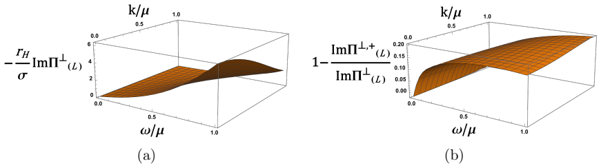
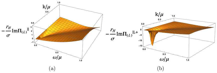
The central claim: at leading order in ω, k, T, μ₃ ≪ μ ≡ √(μ_q²+μ₃²), the charged-current spectral functions of strongly coupled isospin-asymmetric dense matter take the non-Abelian hydrodynamic forms ImΠ^±_⊥ = −Σω and ImΠ^±_∥ = Σω(k²−(ω±μ₃)²)/((ω±μ₃)²+(r_H/2)²k⁴), with Σ = N_c(Mℓ)³w₀²/(8r_H). The isospin background enters only through the shifted frequencies ω±μ₃ and through the horizon radius r_H(μ). The same leading forms hold for ω, k ≪ T ≪ μ and for T ≪ ω, k ≪ μ, so hydrodynamics extends to the hard scale. The paper further claims the extended approximation ImΠ^±_∥ ≈ −Σμ(ω/μ)^{2Δ−1}((ω±μ₃)²−k²)/((ω±μ₃)²+Dk⁴), with Δ = ½+½√(1+r_H²k²/3−r_H²μ₃²/9), which resums low-ω logarithms and capture
What carries the argument
The load-bearing apparatus is the near-extremal matching calculation: the bulk is split into an outer region where the fluctuation equations reduce to radial conservation laws and an inner region near the horizon where they become scalar equations in AdS₂-Schwarzschild, joined by matching the infalling AdS₂ solution to the outer solution. The matching produces the two constitutive constants Σ (conductivity) and D = r_H/2 (diffusivity) from horizon data alone. The second piece is the holographic product formula of reference [23] as applied in reference [11]: it rewrites the spectral function as the KMS-weighted product over poles of the two-sided correlator, which in the T→0 limit converts th
Load-bearing premise
The longitudinal 'extended hydrodynamic' improvement assumes the two-sided correlator has at most finitely many zeroes so the product formula applies — the paper states this assumption in §7 and concedes in §1.1 that a rigorous proof for the longitudinal sector is missing, since its Schrödinger potential is singular in the bulk (appendix J); the transverse channel, whose potential is regular, is not affected.
What would settle it
Compute the exact two-sided longitudinal correlator of the same holographic model at very low T/μ and count its zeroes for momenta up to where the hydro-like pole crosses the AdS₂ levels: an infinite set of zeroes — the known obstruction to the product formula — would invalidate the longitudinal extended approximation and require a modified representation. Independently, the leading-order claim has a sharp kinematic signature: the longitudinal spectral peak and pole must track ω = ∓μ₃ − i(r_H/2)k², shifting linearly with μ₃ at fixed k; a numerical calculation or an analogue measurement of char
If this is right
- Charged-current spectral functions — the inputs to neutrino-emission and -absorption rates in dense matter — become two-constant predictions (Σ, D) in the near-extremal regime, needing no detailed microscopic input beyond the equation of state.
- The validity of the hydrodynamic description extends from ω, k ≪ T ≪ μ to T ≪ ω, k ≪ μ for these correlators, so fluid dynamics remains predictive when frequencies and momenta exceed the temperature.
- A nonzero isospin chemical potential shifts the diffusive pole to ω = ∓μ₃ − iDk² and lowers the infrared scaling dimension to 2Δ(k,μ₃)−1; both effects are confirmed in the quasi-normal-mode spectrum.
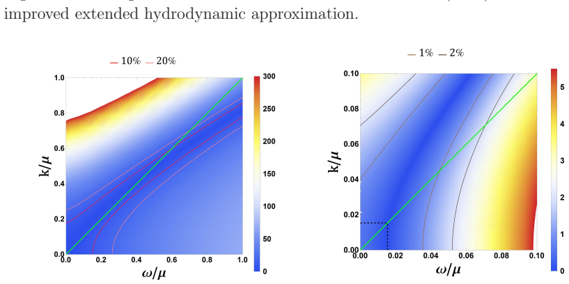
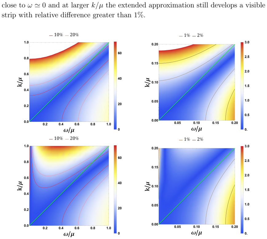
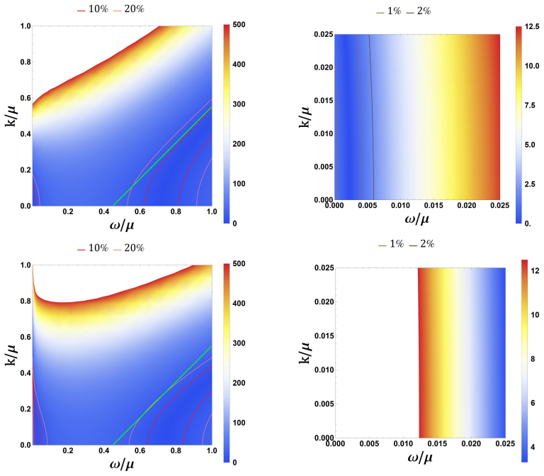
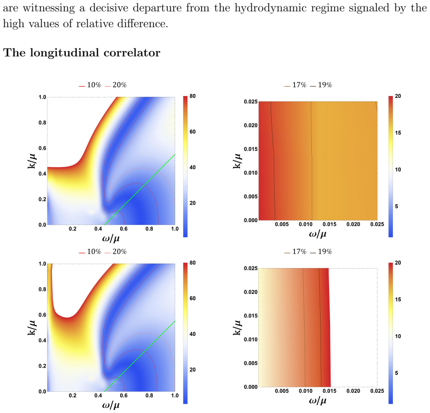
- The extended hydrodynamic approximation improves on plain hydrodynamics mainly near ω = 0, with integrated relative differences at the few-percent level in the low-frequency corner and roughly 15–25% at ω/μ = k/μ = 1/2 for μ_q/T = 65, and it is the simplest among several IR-based approximations of comparable accuracy.
Where Pith is reading between the lines
- The same matching logic applied to the neutral-current sector, where charged currents couple to stress-energy and baryon density, would predict coupled diffusive and sound-like modes; one can test whether the extended regime opens there too, which matters for a complete neutrino-opacity picture.
- Because the longitudinal extended approximation rests on the finite-zeroes assumption, a direct numerical census of the zeroes of the two-sided longitudinal correlator as k increases — including where the hydro-like pole crosses the AdS₂ levels — would either certify or modify formula (7.15); this is the most direct stress test of the paper's advertised improvement.
- The two-constant structure suggests a parameter-free cross-check: if the same μ, T scan were computed with a different bulk action (for instance with Chern–Simons terms or DBI flavor kinetics added), the value of Σ would change but the functional form of both approximations should persist — a signature of the near-extremal mechanism rather than of the specific model.
Editorial analysis
A structured set of objections, weighed in public.
Referee Report
Summary. This paper studies the two-point functions of the charged (U(1)_{I_3}-rotated) components of the SU(2) flavour currents in a strongly coupled dense holographic medium at finite quark and isospin chemical potentials μ_q and μ₃, described by an AdS_5–Reissner-Nordström black hole in an Einstein–Yang-Mills theory. The non-Abelian hydrodynamic form of the charged-current correlators is derived (Section 2), including the shifted Ward identity k±_μ ⟨J^{μ,±}J^{ν,∓}⟩ and the diffusive mode ω = ∓μ₃ − iDk². The holographic spectral functions are then computed from linearized Yang-Mills fluctuations (Section 4). The central technical result (Section 5) is a matched-asymptotic-expansion calculation in the near-extremal regime ω,k,T,μ₃ ≪ μ, which shows that the spectral functions reduce at leading order to the hydrodynamic forms ImΠ^±_⊥ = −Σω and ImΠ^±_∥ = Σω(k²−(ω±μ₃)²)/((ω±μ₃)²+D²k⁴), with Σ = N_c(Mℓ)³w₀²/(8r_H) and D = r_H/2 (Eqs. 5.20–5.21, 5.30–5.31). This generalizes earlier μ₃ = 0 results and supports the claim that the hydrodynamic regime extends to T ≪ ω,k ≪ μ. The paper further applies the holographic product formula (Section 7) to propose an extended hydrodynamic approximation (Eqs. 7.14–7.15) that resums the low-frequency AdS₂ scaling with a momentum-dependent IR dimension Δ(k,μ₃), and verifies both approximations against exact numerical correlators for μ_q/T ∈ {10⁴,65,5} and μ₃/μ_q ∈ {0,−0.1,−0.5} (Section 8 and Appendices L–O).
Significance. The paper's principal contribution is the parameter-free matching computation of Section 5, which derives the non-Abelian hydrodynamic spectral functions (1.2)–(1.3) with Σ and D given by (5.21) and (5.31) directly from the fluctuation equations: the hydrodynamic functional forms are derived independently in Section 2, so the agreement is not obtained by adjusting any parameter to the correlators. If correct, this establishes at leading order that the hydrodynamic description of charged currents — the input to neutrino transport rates in isospin-asymmetric dense matter — extends into the regime T ≪ ω,k,μ₃ ≪ μ. The numerical programme is extensive and well documented: exact spectral functions, quasi-normal-mode spectra, and integrated coarse- and fine-grained relative-difference tables over three densities and three isospin asymmetries (Appendices L–O). The paper is also transparent about the status of its assumptions, explicitly flagging in §1.1 and §7 that the product formula has not been proven for the longitudinal sector. The main caveat — the conditional status of the extended hydrodynamic approximation — is discussed in Major Comment 1; it does not affect the leading-order mat
major comments (2)
- [§7, Eq. (7.5); App. J, Eq. (J.14)] The longitudinal extended-hydrodynamic approximation (7.15) rests on the product formula (7.5), which assumes the longitudinal two-sided correlator has at most finitely many zeroes; the authors state this in §1.1 and §7. This is not a formality: V_∥ is singular where Ω±(r)=0 (Eq. J.14), and for real |ω|<|μ₃| such a point lies in the integration domain, whereas the product formula is proven for regular potentials. A singular potential can generate infinitely many zeroes, in which case (7.5) and (7.15) would fail. The §8 numerics (Tables 5–8) are supportive, but Appendix H shows other IR-based approximations achieve similar accuracy, so they do not select the product-formula mechanism. The §5 matching result is unaffected. Please state the conditional status of (7.15) in the abstract/conclusions, and either analyze the zero structure of the longitudinal two-sided correlator or label (7.15)
- [§7, Eqs. (7.11),(7.15); §6.3] The approximation (7.15) keeps only one hydro-like pole pair in its denominator, but the QNM analysis of §6.3 (Figs. 8–9) shows that a second hydro-like pole emerges at finite momentum in each charged correlator; the paper notes after (7.11) that 'there should be four factors in the denominator of (7.11) instead of two'. The missing poles become relevant at k ≃ √(μT), inside the near-extremal regime, so the abstract's wording that the approximation captures 'both hydrodynamic-like poles' is only accurate at leading order. Please qualify (7.15) as the leading-order truncation, with the second hydro-like pole entering at next-to-leading order.
minor comments (5)
- [Abstract; §1.1] The conditional status of the longitudinal extended-hydrodynamic result (the assumed product formula) is flagged in §1.1 and §7 but not in the abstract, which presents Eqs. (1.18)–(1.19) as obtained. Suggest adding a sentence in the abstract noting that the longitudinal application of the product formula relies on an unproven assumption.
- [Fig. 17 caption] In the caption of Figure 17, the right panel is referred to as '(left panel 17b)'; it should read '(right panel 17b)'.
- [§7, Eq. (7.6)] The KMS relation (7.6) uses the shifted time-translation generator K = H − μ₃Q₃. This convention is important for the definition of frequency in the presence of μ₃; the current discussion is adequate, but a one-sentence reminder of the convention where the spectral functions are plotted would help readers.
- [Abstract; §1.1] The abstract's statement that 'the traditional regime of validity of standard hydrodynamics extends...' could be read as a statement about fully non-linear hydrodynamics. Section 1 correctly emphasizes that only the linearized two-point functions are established; consider aligning the abstract's wording with this qualification.
- [Throughout] Minor typographical/grammatical slips should be corrected in a final pass: e.g., 'The right plots shows a subregion', 'The observables (l)ij is a 4×4 matrix', and the repeated 'we consider' phrasing around Eqs. (8.2)–(8.3).
Circularity Check
No significant circularity: the holographic-to-hydrodynamic matching is derived, not fitted; the longitudinal product-formula extension is an admitted unproven assumption, not a circular reduction.
full rationale
The central derivation is self-contained. Non-Abelian hydrodynamic correlators (2.93)-(2.94) are obtained from linearized covariant conservation and constitutive relations, with Σ and D left as undetermined microscopic coefficients. The holographic spectral functions are then computed from the bulk fluctuation equations (4.8) and (4.15), and the leading-order near-extremal results (5.20) and (5.30) are matched to the hydrodynamic forms, giving Σ = N_c(Mℓ)^3 w_0^2/(8 r_H) and D = r_H/2. These constants are derived analytically from the background/horizon data; they are not adjusted to match the numerical correlators. The numerical verification in section 8 uses exact solutions of the full fluctuation equations described in appendix K, so it is an external check of the approximations rather than a re-use of fitted inputs. The extended hydrodynamic approximation (7.14)-(7.15) is based on the product formula of [23] and the zero-temperature IR scaling; its parameters (Σ, D, Δ(k,μ3)) are again computed, not fitted. The only load-bearing caveat is the extension to the longitudinal sector, where the Schrödinger potential is singular at points where Ω±(r)=0 (J.14). The authors state the assumption explicitly in §7: 'we only assume that the longitudinal two-sided correlator has at most a finite number of zeroes', and in §1.1 they acknowledge that 'a rigorous proof that the results of [11] apply to the longitudinal sector in the non-Abelian case would require further investigation.' This is an admitted unproven assumption and a possible correctness gap, not circularity: no equation of the extended hydrodynamic approximation reduces by construction to the correlator it is meant to reproduce, and no parameter is fitted to the predicted quantity. The admitted gap should be weighed as a correctness risk, but it does not raise the circularity score.
Axiom & Free-Parameter Ledger
free parameters (2)
- Bulk couplings (Mℓ)³ and w₀ =
(Mℓ)³ = 13/(6·45π²); w₀²(Mℓ)³ = 2/(3π²); numerics use N_c = 3, ℓ = 1, w₀ = 6√(5/13) ≈ 3.72
- Scan points μ_q/T and μ₃/μ_q =
μ_q/T ∈ {10⁴, 65, 5}; μ₃/μ_q ∈ {0, -0.1, -0.5}
axioms (7)
- domain assumption AdS/CFT correspondence with the standard holographic dictionary (Son-Starinets infalling prescription) for retarded two-point functions
- domain assumption Veneziano large-N limit (N_c, N_f → ∞ with N_f/N_c fixed) with classical bulk; toy model with conformal glue, no chiral symmetry breaking, no pions
- domain assumption The U(1)_V × SU(2)_V symmetric AdS₅-RN solution with charges μ_q, μ₃ is the dominant saddle in the studied regime
- domain assumption No Chern-Simons terms: C_abc = C = β = γ = 0 (no chiral anomalies)
- domain assumption The canonical boundary time-translation is K = H - μ₃Q₃, which fixes the KMS relation (7.6) and the meaning of ω
- ad hoc to paper The product formula of [23] applies to the charged two-sided correlators with at most finitely many zeroes in the longitudinal sector
- standard math Matched-asymptotics structure: inner AdS₂-Schwarzschild and outer conservation-equation regions with an overlap window (requires k ≪ μ)
read the original abstract
Flavor-current correlators are studied in strongly-coupled dense (holographic) matter, at finite quark chemical potential $\mu_q$ and finite isospin asymmetry. The non-Abelian hydrodynamic description of the charged currents is derived in the presence of an isospin chemical potential $\mu_3$. The two-point correlators of charged currents are then computed holographically at finite quark and isospin chemical potentials. In the near-extremal hydrodynamic regime, $\omega, k, T, \mu_3 \ll \mu \equiv \sqrt{\mu_q^2+\mu_3^2}$, relevant for cold strongly coupled matter, the IR properties of the correlators are studied. It is shown that in this regime, the correlators agree with the non-Abelian hydrodynamic predictions. Therefore, the traditional regime of validity of standard hydrodynamics extends beyond $\omega, k \ll T \ll \mu$ to the so-called extended hydrodynamic regime $T\ll \omega, k \ll \mu$. The holographic product formula is applied to the present non-Abelian system, and is used to propose an extended hydrodynamic approximation capturing both hydrodynamic-like poles and the leading effect of AdS$_2$ poles, by resumming the low-$\omega$ logarithms. The results are verified through a detailed numerical analysis of the exact correlators and quasi-normal mode spectrum.
Figures














Reference graph
Works this paper leans on
-
[1]
Shear Modes, Criticality and Extremal Black Holes,
M. Edalati, J. I. Jottar and R. G. Leigh,“Shear Modes, Criticality and Extremal Black Holes,” JHEP04, 075 (2010) ; [ArXiv:1001.0779][hep-th]
Pith/arXiv arXiv 2010
-
[2]
Transport Coefficients at Zero Temperature from Extremal Black Holes,
M. Edalati, J. I. Jottar and R. G. Leigh,“Transport Coefficients at Zero Temperature from Extremal Black Holes,” JHEP01, 018 (2010) ; [ArXiv:0910.0645][hep-th]
Pith/arXiv arXiv 2010
-
[3]
Holography and the sound of criticality,
M. Edalati, J. I. Jottar and R. G. Leigh,“Holography and the sound of criticality,” JHEP10, 058 (2010) ; [ArXiv:1005.4075][hep-th]
Pith/arXiv arXiv 2010
-
[4]
Bosonic excitations of theAdS 4 Reissner-Nordstrom black hole,
R. A. Davison and N. K. Kaplis,“Bosonic excitations of theAdS 4 Reissner-Nordstrom black hole,” JHEP12, 037 (2011) ; [ArXiv:1111.0660][hep-th]
Pith/arXiv arXiv 2011
-
[5]
Shear channel correlators from hot charged black holes,
D. K. Brattan and S. A. Gentle,“Shear channel correlators from hot charged black holes,” JHEP04, 082 (2011) ; [ArXiv:1012.1280][hep-th]
Pith/arXiv arXiv 2011
-
[6]
Hydrodynamics of cold holographic matter,
R. A. Davison and A. Parnachev,“Hydrodynamics of cold holographic matter,” JHEP06, 100 (2013) ; [ArXiv:1303.6334][hep-th]
Pith/arXiv arXiv 2013
-
[7]
Hydrodynamic Diffusion and Its Breakdown near AdS2 Quantum Critical Points,
D. Arean, R. A. Davison, B. Gout´ eraux and K. Suzuki,“Hydrodynamic Diffusion and Its Breakdown near AdS2 Quantum Critical Points,” Phys. Rev. X11(2021) no.3, 031024. [ArXiv:2011.12301][hep-th]
Pith/arXiv arXiv 2021
-
[8]
Near-Extremal Fluid Mechanics,
U. Moitra, S. K. Sake and S. P. Trivedi,“Near-Extremal Fluid Mechanics,” JHEP 02(2021), 021 ; [ArXiv:2005.00016] [hep-th]
Pith/arXiv arXiv 2021
-
[9]
Holographic neutrino transport in dense strongly-coupled matter,
M. J¨ arvinen, E. Kiritsis, F. Nitti and E. Pr´ eau,“Holographic neutrino transport in dense strongly-coupled matter,” JHEP11(2023), 139 ; [ArXiv:2306.00192] [astro-ph.HE]
Pith/arXiv arXiv 2023
-
[10]
Near-extremal holographic charge correlators,
B. Gout´ eraux, D. M. Ramirez, M. Sanchez-Garitaonandia and C. Supiot, “Near-extremal holographic charge correlators,” [ArXiv:2506.11974][hep-th]
-
[11]
Near-extremal hydrodynamics and the holographic product formula,
E. Pr´ eau,“Near-extremal hydrodynamics and the holographic product formula,” [ArXiv:2512.19330][hep-th]
-
[13]
Weak rates in strongly coupled cold quark matter,
C. Hoyos, A. Olzi and D. Rodriguez-Fernandez,“Weak rates in strongly coupled cold quark matter,” JHEP12(2024), 058 [ArXiv:2407.21643][hep-th]
Pith/arXiv arXiv 2024
-
[14]
Universality of the hydrodynamic limit in AdS/CFT and the membrane paradigm,
N. Iqbal and H. Liu,“Universality of the hydrodynamic limit in AdS/CFT and the membrane paradigm,” Phys. Rev. D79, 025023 (2009) ; [ArXiv:0809.3808][hep-th]
Pith/arXiv arXiv 2009
-
[15]
A Non-Fermi Liquid from a Charged Black Hole: A Critical Fermi Ball,
S. S. Lee,“A Non-Fermi Liquid from a Charged Black Hole: A Critical Fermi Ball,” Phys. Rev. D79(2009), 086006 ; [ArXiv:arXiv:0809.3402][hep-th]. – 168 –
Pith/arXiv arXiv 2009
-
[16]
Non-Fermi liquids from holography,
H. Liu, J. McGreevy and D. Vegh,“Non-Fermi liquids from holography,” Phys. Rev. D83(2011), 065029 ; [ArXiv:arXiv:0903.2477][hep-th]
Pith/arXiv arXiv 2011
-
[17]
Low energy effective theory of Fermi surface coupled with U(1) gauge field in 2+1 dimensions,
S. S. Lee,“Low energy effective theory of Fermi surface coupled with U(1) gauge field in 2+1 dimensions,” Phys. Rev. B80(2009) no.16, 165102 ; [ArXiv:0905.4532][cond-mat.str-el]
Pith/arXiv arXiv 2009
-
[18]
Emergent quantum criticality, Fermi surfaces, and AdS(2),
T. Faulkner, H. Liu, J. McGreevy and D. Vegh,“Emergent quantum criticality, Fermi surfaces, and AdS(2),” Phys. Rev. D83, 125002 (2011) ; [ArXiv:0907.2694][hep-th]
Pith/arXiv arXiv 2011
-
[19]
Holography of Charged Dilaton Black Holes,
K. Goldstein, S. Kachru, S. Prakash and S. P. Trivedi,“Holography of Charged Dilaton Black Holes,” JHEP08(2010), 078 ; [ArXiv:0911.3586][hep-th]
Pith/arXiv arXiv 2010
-
[20]
C. Charmousis, B. Gouteraux, B. S. Kim, E. Kiritsis and R. Meyer, JHEP11 (2010), 151; [ArXiv:1005.4690] [hep-th]
Pith/arXiv arXiv 2010
-
[21]
Holographic Fermi and Non-Fermi Liquids with Transitions in Dilaton Gravity,
N. Iizuka, N. Kundu, P. Narayan and S. P. Trivedi,“Holographic Fermi and Non-Fermi Liquids with Transitions in Dilaton Gravity,” JHEP01(2012), 094 [ArXiv:arXiv:1105.1162][hep-th]
Pith/arXiv arXiv 2012
-
[22]
Generalized Holographic Quantum Criticality at Finite Density,
B. Gouteraux and E. Kiritsis,“Generalized Holographic Quantum Criticality at Finite Density,” JHEP12(2011), 036 ; [ArXiv:1107.2116]hep-th]
Pith/arXiv arXiv 2011
-
[23]
M. Dodelson, C. Iossa, R. Karlsson and A. Zhiboedov,“A thermal product formula,” JHEP01(2024), 036 ; [ArXiv:2304.12339][hep-th]
Pith/arXiv arXiv 2024
-
[24]
Entanglement in Strongly- Correlated Quantum Matter
A. Y. Kitaev,“ Entanglement in Strongly- Correlated Quantum Matter”, Talks at KITP, University of California, Santa Barbara,(2015)
2015
-
[25]
Bekenstein-Hawking Entropy and Strange Metals,
S. Sachdev,“Bekenstein-Hawking Entropy and Strange Metals,” Phys. Rev. X5 (2015) no.4, 041025 ; [ArXiv:1506.05111] [hep-th]
Pith/arXiv arXiv 2015
-
[26]
Remarks on the Sachdev-Ye-Kitaev model,
J. Maldacena and D. Stanford,“Remarks on the Sachdev-Ye-Kitaev model,” Phys. Rev. D94(2016) no.10, 106002 ; [ArXiv:1604.07818] [hep-th]
Pith/arXiv arXiv 2016
-
[27]
K. Jensen,“Chaos in AdS 2 Holography,” Phys. Rev. Lett.117(2016) no.11, 111601 ; [ArXiv:1605.06098][hep-th]
Pith/arXiv arXiv 2016
-
[28]
Conformal symmetry and its breaking in two dimensional Nearly Anti-de-Sitter space,
J. Maldacena, D. Stanford and Z. Yang,“Conformal symmetry and its breaking in two dimensional Nearly Anti-de-Sitter space,” PTEP2016(2016) no.12, 12C104 [ArXiv:1606.01857][hep-th]
Pith/arXiv arXiv 2016
-
[29]
Solvable models of quantum black holes: a review on Jackiw–Teitelboim gravity,
T. G. Mertens and G. J. Turiaci,“Solvable models of quantum black holes: a review on Jackiw–Teitelboim gravity,” Living Rev. Rel.26(2023) no.1, 4 [ArXiv:2210.10846] [hep-th]
Pith/arXiv arXiv 2023
-
[30]
Solving the Schwarzian via the Conformal Bootstrap,
T. G. Mertens, G. J. Turiaci and H. L. Verlinde,“Solving the Schwarzian via the Conformal Bootstrap,” JHEP08(2017), 136 ; [ArXiv:1705.08408] [hep-th]. – 169 –
Pith/arXiv arXiv 2017
-
[31]
A. Kanargias, E. Kiritsis, S. Murthy, O. Papadoulaki and A. P. Porfyriadis, [ArXiv:2512.20443][hep-th]; to appear in JHEP
-
[32]
X.-H. Ge, S.-K. Jian, Y.-L. Wang, Z.-Y. Xian and H. Yao,Violation of the viscosity/entropy bound in translationally invariant non-Fermi liquids, Phys. Rev. Res.2(2020) 023366 , [1810.00669]
Pith/arXiv arXiv 2020
-
[33]
One-loop Corrected Holographic Shear Viscosity to Entropy Density Ratio at Low Temperatures,
L. A. Pando Zayas and J. Zhang,“One-loop Corrected Holographic Shear Viscosity to Entropy Density Ratio at Low Temperatures,” [ArXiv:2510.16100] [hep-th]
-
[34]
Quantum Corrections toη/sfrom JT Gravity,
S. Cremonini, L. Li, X. L. Liu and J. Nian,“Quantum Corrections toη/sfrom JT Gravity,” [ArXiv:2510.21602] [hep-th]
-
[35]
B. Gout´ eraux, D. M. Ramirez and C. Supiot,“Schwarzian quantum corrections to shear correlators of the near-extremal Reissner-Nordstr¨ om-AdS black hole,” [ArXiv:2512.19642] [hep-th]
-
[36]
Classical Glasses, Black Holes, and Strange Quantum Liquids,
D. Facoetti, G. Biroli, J. Kurchan and D. R. Reichman,“Classical Glasses, Black Holes, and Strange Quantum Liquids,” Phys. Rev. B100(2019) no.20, 205108 ; [ArXiv:1906.09228] [hep-th]
Pith/arXiv arXiv 2019
-
[37]
Semi-local Quantum Criticality and the Instability of Extremal Planar Horizons,
S. E. Gralla, A. Ravishankar and P. Zimmerman,“Semi-local Quantum Criticality and the Instability of Extremal Planar Horizons,” JHEP12(2018), 087 ; [ArXiv:1808.07053] [hep-th]
Pith/arXiv arXiv 2018
-
[38]
Horizon Instability of Extremal Black Holes,
S. Aretakis,“Horizon Instability of Extremal Black Holes,” Adv. Theor. Math. Phys. 19(2015), 507-530 ; [ArXiv:1206.6598] [gr-qc]
Pith/arXiv arXiv 2015
-
[39]
Many-Body Chaos in the Sachdev-Ye-Kitaev Model,
B. Kobrin, Z. Yang, G. D. Kahanamoku-Meyer, C. T. Olund, J. E. Moore, D. Stanford and N. Y. Yao,“Many-Body Chaos in the Sachdev-Ye-Kitaev Model,” [ArXiv:10.1103/PhysRevLett.126.030602]Phys. Rev. Lett.126(2021) no.3, 030602 ; [ArXiv:2002.05725] [hep-th]
Pith/arXiv arXiv 2021
-
[40]
Anti-de Sitter space, thermal phase transition, and confinement in gauge theories,
E. Witten,“Anti-de Sitter space, thermal phase transition, and confinement in gauge theories,” Adv. Theor. Math. Phys.2(1998), 505-532 ; [ArXiv:hep-th/9803131]
Pith/arXiv arXiv 1998
-
[41]
Low energy hadron physics in holographic QCD,
T. Sakai and S. Sugimoto,“Low energy hadron physics in holographic QCD,” Prog. Theor. Phys.113(2005), 843-882 ; [ArXiv:hep-th/0412141]
Pith/arXiv arXiv 2005
-
[42]
Exploring improved holographic theories for QCD: Part I,
U. Gursoy and E. Kiritsis,“Exploring improved holographic theories for QCD: Part I,” JHEP02(2008), 032 ; [ArXiv:0707.1324/hep-th]; U. Gursoy, E. Kiritsis and F. Nitti,“Exploring improved holographic theories for QCD: Part II,” JHEP02(2008), 019 [ArXiv:0707.1349/ [hep-th]]
Pith/arXiv arXiv 2008
-
[43]
S. S. Gubser, A. Nellore, S. S. Pufu and F. D. Rocha,“Thermodynamics and bulk viscosity of approximate black hole duals to finite temperature quantum chromodynamics,” Phys. Rev. Lett.101, 131601 (2008) ; [ArXiv:0804.1950][hep-th]. – 170 –
Pith/arXiv arXiv 2008
-
[44]
Bulk viscosity of strongly coupled plasmas with holographic duals,
S. S. Gubser, S. S. Pufu and F. D. Rocha,“Bulk viscosity of strongly coupled plasmas with holographic duals,” JHEP08, 085 (2008) ; [ArXiv:0806.0407][hep-th]
Pith/arXiv arXiv 2008
-
[45]
Deconfinement and Gluon Plasma Dynamics in Improved Holographic QCD,
U. Gursoy, E. Kiritsis, L. Mazzanti and F. Nitti,“Deconfinement and Gluon Plasma Dynamics in Improved Holographic QCD,” Phys. Rev. Lett.101(2008), 181601 ; [ArXiv:0804.0899] [hep-th]; “Holography and Thermodynamics of 5D Dilaton-gravity,” JHEP05(2009), 033 ; [ArXiv:0812.0792][hep-th]
Pith/arXiv arXiv 2008
-
[46]
Thermal Transport and Drag Force in Improved Holographic QCD,
U. Gursoy, E. Kiritsis, G. Michalogiorgakis and F. Nitti,“Thermal Transport and Drag Force in Improved Holographic QCD,” JHEP12, 056 (2009) ; [ArXiv:0906.1890][hep-ph]
Pith/arXiv arXiv 2009
-
[47]
Langevin diffusion of heavy quarks in non-conformal holographic backgrounds,
U. Gursoy, E. Kiritsis, L. Mazzanti and F. Nitti,“Langevin diffusion of heavy quarks in non-conformal holographic backgrounds,” JHEP12, 088 (2010) ; [ArXiv:1006.3261][hep-th]
Pith/arXiv arXiv 2010
-
[48]
Holographic Models for QCD in the Veneziano Limit,
M. Jarvinen and E. Kiritsis,“Holographic Models for QCD in the Veneziano Limit,” JHEP03(2012), 002 ; [ArXiv:1112.1261] [hep-ph]
Pith/arXiv arXiv 2012
-
[49]
On finite-temperature holographic QCD in the Veneziano limit,
T. Alho, M. J¨ arvinen, K. Kajantie, E. Kiritsis and K. Tuominen,“On finite-temperature holographic QCD in the Veneziano limit,” JHEP01(2013), 093 ; [ArXiv:1210.4516] [hep-ph]
Pith/arXiv arXiv 2013
-
[50]
V-QCD: Spectra, the dilaton and the S-parameter,
D. Arean, I. Iatrakis, M. J¨ arvinen and E. Kiritsis,“V-QCD: Spectra, the dilaton and the S-parameter,” Phys. Lett. B720(2013), 219-223 ; [ArXiv:1211.6125] [hep-ph]; “The discontinuities of conformal transitions and mass spectra of V-QCD,” JHEP 11(2013), 068 ; [ArXiv:1309.2286] [hep-ph]
Pith/arXiv arXiv 2013
-
[51]
A holographic model for QCD in the Veneziano limit at finite temperature and density,
T. Alho, M. J¨ arvinen, K. Kajantie, E. Kiritsis, C. Rosen and K. Tuominen,“A holographic model for QCD in the Veneziano limit at finite temperature and density,” JHEP04(2014), 124 ; erratum: JHEP02(2015), 033 ; [ArXiv:1312.5199] [hep-ph]
Pith/arXiv arXiv 2014
-
[52]
Massive holographic QCD in the Veneziano limit,
M. J¨ arvinen,“Massive holographic QCD in the Veneziano limit,” JHEP07(2015), 033; [ArXiv:1501.07272] [hep-ph]
Pith/arXiv arXiv 2015
-
[53]
CP-odd sector andθdynamics in holographic QCD,
D. Arean, I. Iatrakis, M. Jarvinen and E. Kiritsis,“CP-odd sector andθdynamics in holographic QCD,” Phys. Rev. D96(2017) no.2, 026001 ; [ArXiv:1609.08922] [hep-ph]
Pith/arXiv arXiv 2017
-
[54]
Cool baryon and quark matter in holographic QCD,
T. Ishii, M. J¨ arvinen and G. Nijs,“Cool baryon and quark matter in holographic QCD,” JHEP07, 003 (2019) ; [ArXiv:1903.06169][hep-ph]
Pith/arXiv arXiv 2019
-
[55]
Holographic QCD in the Veneziano limit and neutron stars,
N. Jokela, M. J¨ arvinen and J. Remes,“Holographic QCD in the Veneziano limit and neutron stars,” JHEP03, 041 (2019) ; [ArXiv:1809.07770][hep-ph]
Pith/arXiv arXiv 2019
-
[56]
The V-QCD baryon : numerical solution and baryon spectrum,
M. J¨ arvinen, E. Kiritsis, F. Nitti and E. Pr´ eau,“The V-QCD baryon : numerical solution and baryon spectrum,” [ArXiv:2212.06747] [hep-th]; – 171 – “Tachyon-dependent Chern-Simons terms and the V-QCD baryon,” JHEP12 (2022), 160; [ArXiv:2209.05868] [hep-th]
Pith/arXiv arXiv 2022
-
[57]
An AdS/QCD model from Sen ’s tachyon action,
I. Iatrakis, E. Kiritsis and A. Paredes,“An AdS/QCD model from Sen ’s tachyon action,” Phys. Rev. D81(2010), 115004 ; [ArXiv:1003.2377] [hep-ph]
Pith/arXiv arXiv 2010
-
[58]
An AdS/QCD model from tachyon condensation: II,
I. Iatrakis, E. Kiritsis and A. Paredes,“An AdS/QCD model from tachyon condensation: II,” JHEP11(2010), 123 ; [ArXiv:1010.1364] [hep-ph]
Pith/arXiv arXiv 2010
-
[59]
Neutron stars 1: Equation of state and structure,
P. Haensel, A. Y. Potekhin and D. G. Yakovlev,“Neutron stars 1: Equation of state and structure,” Astrophys. Space Sci. Libr.326, pp.1-619 (2007) Springer, 2007
2007
-
[60]
S. S. Gubser,“Drag force in AdS/CFT,” Phys. Rev. D74(2006), 126005 ; [ArXiv:hep-th/0605182] [hep-th]
Pith/arXiv arXiv 2006
-
[61]
QCD at finite isospin density: From pion to quark - anti-quark condensation,
D. T. Son and M. A. Stephanov,“QCD at finite isospin density: From pion to quark - anti-quark condensation,” Phys. Atom. Nucl.64(2001), 834-842 ; [ArXiv:hep-ph/0011365]
Pith/arXiv arXiv 2001
-
[62]
Phases and phase transitions of U(1)×SU(2) symmetric holographic matter,
M. J¨ arvinen, E. Kiritsis, F. Nitti and E. Pr´ eau,“Phases and phase transitions of U(1)×SU(2) symmetric holographic matter,” JHEP03(2025), 005 ; [ArXiv:2409.04630] [hep-th]
Pith/arXiv arXiv 2025
-
[63]
Colorful horizons with charge in anti-de Sitter space,
S. S. Gubser,“Colorful horizons with charge in anti-de Sitter space,” Phys. Rev. Lett.101(2008), 191601 ; [ArXiv:0803.3483] [hep-th]
Pith/arXiv arXiv 2008
-
[64]
The Gravity dual of a p-wave superconductor,
S. S. Gubser and S. S. Pufu,“The Gravity dual of a p-wave superconductor,” JHEP 11(2008), 033 ; [ArXiv:0805.2960] [hep-th]
Pith/arXiv arXiv 2008
-
[65]
Rho meson condensation at finite isospin chemical potential in a holographic model for QCD,
O. Aharony, K. Peeters, J. Sonnenschein and M. Zamaklar,“Rho meson condensation at finite isospin chemical potential in a holographic model for QCD,” JHEP02(2008), 071 ; [ArXiv:0709.3948][hep-th]
Pith/arXiv arXiv 2008
-
[66]
Perfect fluid theory and its extensions,
R. Jackiw, V. P. Nair, S. Y. Pi and A. P. Polychronakos,“Perfect fluid theory and its extensions,” [ArXiv:hep-th/0004084][hep-th]
-
[67]
Non-Abelian fluid dynamics in Lagrangian formulation,
B. Bistrovic, R. Jackiw, H. Li, V. P. Nair and S. Y. Pi,“Non-Abelian fluid dynamics in Lagrangian formulation,” Phys. Rev. D67, 025013 (2003) ; [ArXiv:hep-th/0210143][hep-th]
Pith/arXiv arXiv 2003
-
[68]
A particle field theorist’s lectures on supersymmetric, non-Abelian fluid mechanics and d-branes,
R. Jackiw,“A particle field theorist’s lectures on supersymmetric, non-Abelian fluid mechanics and d-branes,” [ArXiv:hep-th/0407101][hep-th]
-
[69]
Hydrodynamics of nuclear matter in the chiral limit,
D. T. Son,“Hydrodynamics of nuclear matter in the chiral limit,” Phys. Rev. Lett. 84, 3771–3774 (2000) ; [ArXiv:hep-ph/9912267][hep-ph]
Pith/arXiv arXiv 2000
-
[70]
Pion propagation near the QCD chiral phase transition,
D. T. Son and M. A. Stephanov,“Pion propagation near the QCD chiral phase transition,” Phys. Rev. Lett.88, 202302 (2002) ; [ArXiv:hep-ph/0111100][hep-ph]. – 172 –
Pith/arXiv arXiv 2002
-
[71]
Real-time pion propagation in finite-temperature QCD,
D. T. Son and M. A. Stephanov,“Real-time pion propagation in finite-temperature QCD,” Phys. Rev. D66, 076011 (2002) ; [ArXiv:hep-ph/0204226][hep-ph]
Pith/arXiv arXiv 2002
-
[72]
Holographic nonlinear hydrodynamics from AdS/CFT with multiple/non-Abelian symmetries,
M. Torabian and H. U. Yee,“Holographic nonlinear hydrodynamics from AdS/CFT with multiple/non-Abelian symmetries,” JHEP08, 020 (2009) ; [ArXiv:0903.4894][hep-th]
Pith/arXiv arXiv 2009
-
[73]
Fluid dynamics of R-charged black holes,
J. Erdmenger, M. Haack, M. Kaminski and A. Yarom,“Fluid dynamics of R-charged black holes,” JHEP01, 055 (2009) ; [ArXiv:0809.2488/[hep-th]]
Pith/arXiv arXiv 2009
-
[76]
Relativistic Hydrodynamics with General Anomalous Charges,
Y. Neiman and Y. Oz,“Relativistic Hydrodynamics with General Anomalous Charges,” JHEP03, 023 (2011) ; [ArXiv:1011.5107][hep-th]
Pith/arXiv arXiv 2011
-
[77]
Relativistic CFT Hydrodynamics from the Membrane Paradigm,
C. Eling and Y. Oz,“Relativistic CFT Hydrodynamics from the Membrane Paradigm,” JHEP02, 069 (2011) ; [ArXiv:1010.1290][hep-th]
Pith/arXiv arXiv 2011
-
[78]
Odd Parity Transport In Non-Abelian Superfluids From Symmetry Locking,
C. Hoyos, B. S. Kim and Y. Oz,“Odd Parity Transport In Non-Abelian Superfluids From Symmetry Locking,” JHEP10(2014), 127 [ArXiv:1404.7507][hep-th]
Pith/arXiv arXiv 2014
-
[79]
A New Approach to Non-Abelian Hydrodynamics,
J. J. Fernandez-Melgarejo, S. J. Rey and P. Sur´ owka,“A New Approach to Non-Abelian Hydrodynamics,” JHEP02, 122 (2017) ; [ArXiv:1605.06080][hep-th]
Pith/arXiv arXiv 2017
-
[80]
Theory of non-Abelian superfluid dynamics,
A. Jain,“Theory of non-Abelian superfluid dynamics,” Phys. Rev. D95, 121701 (2017); [ArXiv:1610.05797][hep-th]
Pith/arXiv arXiv 2017
-
[81]
Transport and hydrodynamics in the chiral limit,
E. Grossi, A. Soloviev, D. Teaney and F. Yan,“Transport and hydrodynamics in the chiral limit,” Phys. Rev. D102, 014042 (2020) ; [ArXiv:2005.02885][hep-th]
Pith/arXiv arXiv 2020
-
[82]
Nonabelian fluids and helicities,
H. Nastase and J. Sonnenschein,“Nonabelian fluids and helicities,” JHEP07(2025), 015; [ArXiv:2502.13765] [hep-th]
Pith/arXiv arXiv 2025
-
[83]
Hydrodynamics with Triangle Anomalies,
D. T. Son and P. Surowka,“Hydrodynamics with Triangle Anomalies,” Phys. Rev. Lett.103, 191601 (2009) ; [ArXiv:0906.5044][hep-th]
Pith/arXiv arXiv 2009
discussion (0)
Sign in with ORCID, Apple, or X to comment. Anyone can read and Pith papers without signing in.