The HST/WFC3 Transmission Spectrum of AU Mic b Part I: An Atmosphere Obscured by Contamination and Systematics
Pith reviewed 2026-07-01 03:48 UTC · model grok-4.3
The pith
The transmission spectrum of AU Mic b is dominated by the transit light source effect from its host star's spots, leaving only weak constraints on its atmosphere.
A machine-rendered reading of the paper's core claim, the machinery that carries it, and where it could break.
Core claim
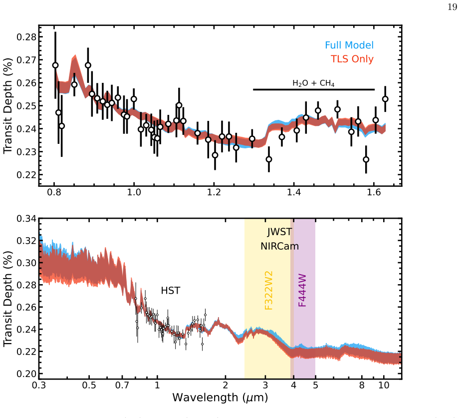
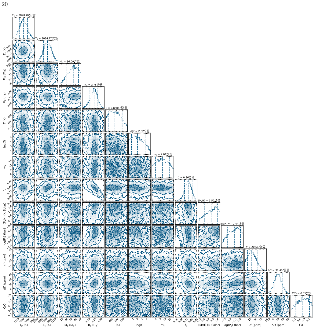
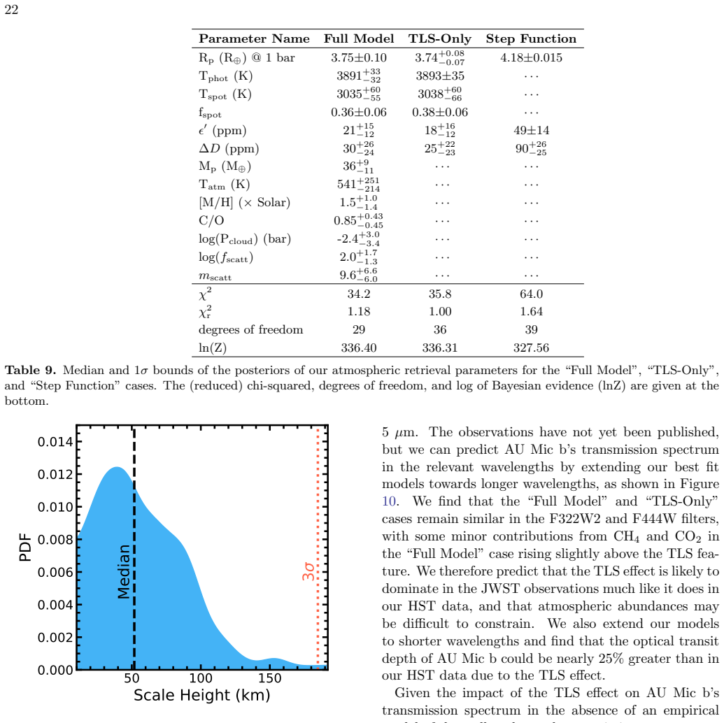
Using decomposition of the out-of-transit stellar SED, the photospheric temperature is 3891±37 K, spot temperature 3020±69 K, and spot filling factor 0.33±0.05. Bayesian atmospheric retrievals indicate the spectrum is dominated by the TLS effect, with weak atmospheric constraints and a preferred scale height of less than 185 km at 3σ. Extrapolation shows TLS dominates atmospheric features at optical and infrared wavelengths.
What carries the argument
The transit light source (TLS) effect, arising from the difference in brightness between the unocculted stellar photosphere and spots during transit, which alters the apparent transit depth.
If this is right
- The TLS effect will dominate the transmission spectrum of AU Mic b at optical and infrared wavelengths.
- The planet's atmosphere has a relatively small scale height, implying limited extent or high mean molecular weight.
- Stellar activity must be carefully modeled to extract atmospheric signals from transmission spectra of active M dwarfs.
- Weak atmospheric constraints mean current data cannot distinguish between different atmospheric compositions for AU Mic b.
Where Pith is reading between the lines
- Similar young planets around active stars may require even more sophisticated corrections for TLS to reveal their atmospheres.
- Future observations at wavelengths where TLS is minimal could still be affected if spot properties vary.
- Improved modeling of stellar variability could enable detection of escaping hydrogen or other features hinted at in prior observations.
Load-bearing premise
The decomposition of the out-of-transit stellar SED accurately captures the photospheric and spot properties that affect the in-transit observations.
What would settle it
An observation of the transmission spectrum at a wavelength where the TLS effect is predicted to be strong but atmospheric features are expected to appear would show a mismatch if the atmospheric signal is detected instead.
Figures
read the original abstract
Young sub-Neptune progenitors around M dwarfs offer an excellent opportunity to probe the formation of their abundant, older cousins. At $\sim$20 Myr and only 9.7 pc away, AU Mic b is an ideal candidate for this effort, with its density and observations of escaping hydrogen pointing to a significant primordial atmosphere. Here we present the 0.8-1.6 $\micron$ transmission spectrum of AU Mic b observed with the Wide Field Camera 3 on the Hubble Space Telescope (HST). We find that HST experienced unstable scanning during its visits, resulting in a variable PSF that dramatically affects the orbit-to-orbit baseline of the observations. While we were able to somewhat mitigate this problem through spectral binning, the effects cannot be completely eliminated, limiting the precision of our results. Our data is further impacted by the intense magnetic activity of AU Mic, which introduced significant rotational variability along with spot crossings and the transit light source (TLS) effect into the light curves and spectrum, respectively. Through decomposition of the out-of-transit stellar SED, we are able to constrain AU Mic's photospheric and spot temperatures to 3891$\pm$37 and 3020$\pm$69 K, respectively, with a spot filling factor of $0.33\pm0.05$. Using Bayesian atmospheric retrievals, we show that the spectrum is dominated by the TLS effect with weak atmospheric constraints, with the data preferring a relatively small scale height of $<$185 km to 3$\sigma$. Extrapolation of our retrieved spectra shows that the TLS effect dominates over atmospheric features at optical and infrared wavelengths.
Editorial analysis
A structured set of objections, weighed in public.
Referee Report
Summary. The manuscript presents the 0.8-1.6 μm HST/WFC3 transmission spectrum of the young sub-Neptune AU Mic b. Unstable scanning produced variable PSF that affects orbit-to-orbit baselines and cannot be fully removed even after spectral binning. Stellar activity introduces rotational variability, spot crossings, and the transit light source (TLS) effect. Decomposition of the out-of-transit stellar SED constrains photospheric temperature to 3891±37 K, spot temperature to 3020±69 K, and spot filling factor to 0.33±0.05. Bayesian atmospheric retrievals indicate that the observed spectrum is dominated by TLS, with only weak atmospheric constraints; the data prefer a scale height <185 km at 3σ. Extrapolation shows TLS dominating atmospheric features at optical and infrared wavelengths.
Significance. If the TLS correction holds, the result provides a concrete demonstration that stellar heterogeneity can mask atmospheric signals in transmission spectra of young planets around active M dwarfs, with direct implications for formation and evolution studies of sub-Neptunes. The work also supplies quantitative limits on the atmospheric scale height under the adopted TLS model.
major comments (2)
- [SED decomposition and TLS correction sections] The central claim that TLS dominates the spectrum (and that the atmosphere prefers scale height <185 km at 3σ) rests on applying the out-of-transit SED-derived parameters (T_phot=3891±37 K, T_spot=3020±69 K, f_spot=0.33±0.05) as the TLS correction during transit. For an active star with known non-uniform spot distribution, these disk-integrated values may not represent the specific photosphere and spots occulted by the planet; no test of this assumption (e.g., via spot-crossing events or multi-epoch comparisons) is described. This is load-bearing for the retrieval results.
- [Data reduction and light-curve modeling sections] The manuscript states that PSF variability from unstable scanning 'cannot be completely eliminated' and limits precision, yet the quantitative impact of residual baseline variations on the retrieved scale-height upper limit and on the TLS-versus-atmosphere decomposition is not assessed (e.g., via injection-recovery or covariance analysis).
minor comments (1)
- [Retrieval setup] Notation for the spot filling factor and its propagation into the retrieval should be clarified; it is introduced as a free parameter but its prior and posterior are not tabulated.
Simulated Author's Rebuttal
We thank the referee for their careful reading and constructive comments, which highlight important assumptions and limitations in our analysis. We address each major comment below and outline revisions to improve clarity and robustness.
read point-by-point responses
-
Referee: [SED decomposition and TLS correction sections] The central claim that TLS dominates the spectrum (and that the atmosphere prefers scale height <185 km at 3σ) rests on applying the out-of-transit SED-derived parameters (T_phot=3891±37 K, T_spot=3020±69 K, f_spot=0.33±0.05) as the TLS correction during transit. For an active star with known non-uniform spot distribution, these disk-integrated values may not represent the specific photosphere and spots occulted by the planet; no test of this assumption (e.g., via spot-crossing events or multi-epoch comparisons) is described. This is load-bearing for the retrieval results.
Authors: We agree that the TLS correction relies on the assumption that the disk-integrated spot parameters derived from the out-of-transit SED are representative of the stellar surface occulted during transit. This is a standard approach when chord-specific constraints are unavailable, but we acknowledge it is load-bearing for the conclusion that TLS dominates. The manuscript notes the presence of spot-crossing events in the light curves, yet these were not quantitatively modeled to adjust the filling factor for the transit chord due to their low signal-to-noise relative to the overall variability. We will revise the relevant sections to explicitly discuss this assumption, its potential systematic uncertainty, and the value of future multi-epoch observations for testing it. This constitutes a partial revision. revision: partial
-
Referee: [Data reduction and light-curve modeling sections] The manuscript states that PSF variability from unstable scanning 'cannot be completely eliminated' and limits precision, yet the quantitative impact of residual baseline variations on the retrieved scale-height upper limit and on the TLS-versus-atmosphere decomposition is not assessed (e.g., via injection-recovery or covariance analysis).
Authors: We agree that a quantitative assessment of residual baseline variations from the unstable scanning would strengthen the robustness claims. While the manuscript already states that these effects limit precision even after binning, we did not perform injection-recovery tests or covariance analysis to propagate their impact specifically onto the scale-height upper limit or the TLS-atmosphere decomposition. We will add such tests in the revised manuscript to evaluate how residual systematics could affect the 3σ preference for scale height <185 km. This will be incorporated as a new subsection. revision: yes
Circularity Check
No significant circularity; sequential fitting of stellar parameters from out-of-transit data followed by independent retrieval
full rationale
The paper decomposes the out-of-transit stellar SED to obtain photospheric/spot temperatures and filling factor, applies a TLS correction derived from those parameters to the transmission spectrum, and then runs Bayesian atmospheric retrievals on the corrected data to constrain scale height. This is a standard forward-modeling sequence with no self-definitional loops, no fitted inputs renamed as predictions, and no load-bearing self-citations or uniqueness theorems in the provided text. The retrieval result (scale height <185 km) is an output of the corrected spectrum rather than a re-expression of the stellar fit inputs. The derivation remains self-contained against external benchmarks.
Axiom & Free-Parameter Ledger
free parameters (4)
- spot filling factor =
0.33±0.05
- photospheric temperature =
3891±37 K
- spot temperature =
3020±69 K
- atmospheric scale height upper limit =
<185 km (3σ)
axioms (1)
- domain assumption Standard assumptions underlying Bayesian atmospheric retrieval codes for transmission spectra (e.g., forward model physics, prior distributions)
Reference graph
Works this paper leans on
-
[1]
2020, AJ, 159, 123, doi: 10.3847/1538-3881/ab4fee
Agol, E., Luger, R., & Foreman-Mackey, D. 2020, AJ, 159, 123, doi: 10.3847/1538-3881/ab4fee
-
[2]
Allard, F., Homeier, D., & Freytag, B. 2012, Philosophical Transactions of the Royal Society of London Series A, 370, 2765, doi: 10.1098/rsta.2011.0269
-
[3]
Asplund, M., Amarsi, A. M., & Grevesse, N. 2021, A&A, 653, A141, doi: 10.1051/0004-6361/202140445 Astropy Collaboration, Robitaille, T. P., Tollerud, E. J., et al. 2013, A&A, 558, A33, doi: 10.1051/0004-6361/201322068 Astropy Collaboration, Price-Whelan, A. M., Sip˝ ocz, B. M., et al. 2018, AJ, 156, 123, doi: 10.3847/1538-3881/aabc4f Astropy Collaboration...
work page internal anchor Pith review doi:10.1051/0004-6361/202140445 2021
-
[4]
Barat, S., D´ esert, J.-M., Vazan, A., et al. 2024a, Nature Astronomy, 8, 899, doi: 10.1038/s41550-024-02257-0
-
[5]
Barat, S., D´ esert, J.-M., Goyal, J. M., et al. 2024b, A&A, 692, A198, doi: 10.1051/0004-6361/202451127
-
[6]
Barat, S., D´ esert, J.-M., Mukherjee, S., et al. 2025, AJ, 170, 165, doi: 10.3847/1538-3881/adec89
-
[7]
Barclay, T., Kostov, V. B., Col´ on, K. D., et al. 2021, AJ, 162, 300, doi: 10.3847/1538-3881/ac2824
-
[8]
Bean, J. L., Raymond, S. N., & Owen, J. E. 2021, Journal of Geophysical Research (Planets), 126, e06639, doi: 10.1029/2020JE006639
-
[9]
Benneke, B., Wong, I., Piaulet, C., et al. 2019, ApJL, 887, L14, doi: 10.3847/2041-8213/ab59dc
-
[10]
Berdyugina, S. V. 2005, Living Reviews in Solar Physics, 2, 8, doi: 10.12942/lrsp-2005-8
-
[11]
P., Jankowiak, M., et al
Bingham, E., Chen, J. P., Jankowiak, M., et al. 2019, J. Mach. Learn. Res., 20, 28:1. http://jmlr.org/papers/v20/18-403.html
2019
-
[12]
Blunt, S., Carvalho, A., David, T. J., et al. 2023, AJ, 166, 62, doi: 10.3847/1538-3881/acde78
-
[13]
L., Reefe, M., Plavchan, P., et al
Cale, B. L., Reefe, M., Plavchan, P., et al. 2021, AJ, 162, 295, doi: 10.3847/1538-3881/ac2c80
-
[14]
A., Plavchan, P., Villarreal D’Angelo, C., & Hazra, G
Carolan, S., Vidotto, A. A., Plavchan, P., Villarreal D’Angelo, C., & Hazra, G. 2020, MNRAS, 498, L53, doi: 10.1093/mnrasl/slaa127
-
[15]
Cherubim, C., Wordsworth, R., Bower, D. J., et al. 2025, ApJ, 983, 97, doi: 10.3847/1538-4357/adbca9
-
[16]
I., Plavchan, P., Berta-Thompson, Z., et al
Collins, K. I., Plavchan, P., Berta-Thompson, Z., et al. 2026, https://arxiv.org/abs/2602.05168
-
[17]
2024, AJ, 168, 227, doi: 10.3847/1538-3881/ad7aef de Wit, J., & Seager, S
Coulombe, L.-P., Roy, P.-A., & Benneke, B. 2024, AJ, 168, 227, doi: 10.3847/1538-3881/ad7aef de Wit, J., & Seager, S. 2013, Science, 342, 1473, doi: 10.1126/science.1245450
-
[18]
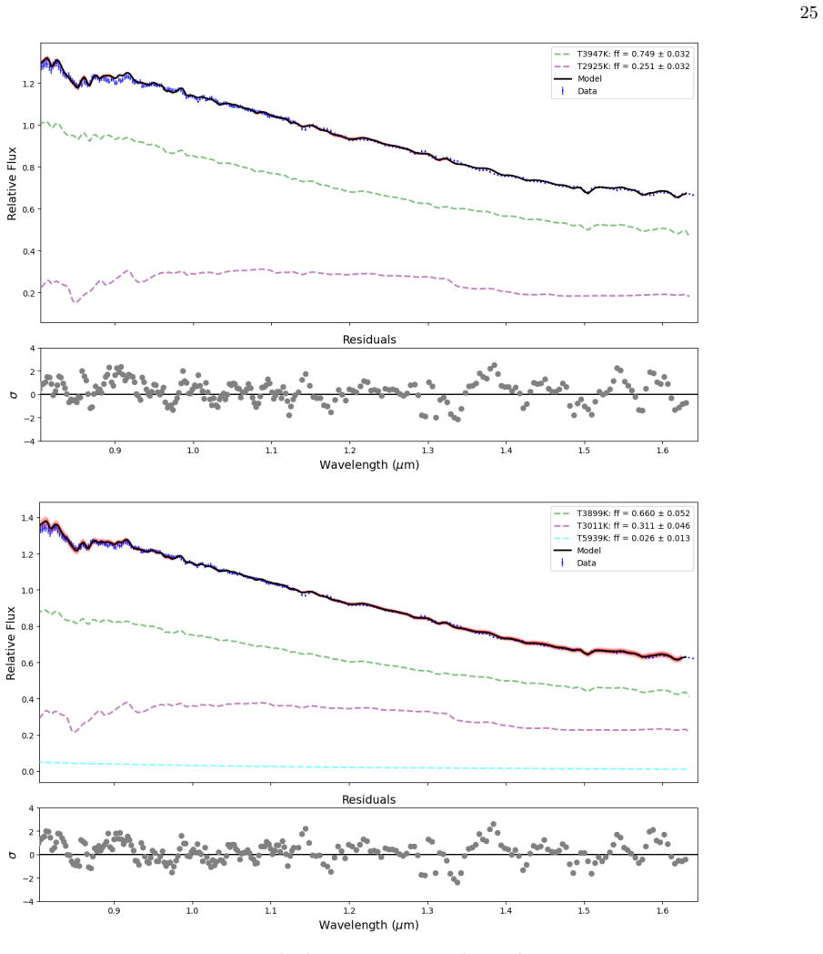
Deming, D., Wilkins, A., McCullough, P., et al. 2013, ApJ, 774, 95, doi: 10.1088/0004-637X/774/2/95 25 Figure 13.SED decomposition with 2 temperature (top) and 3 temperature (bottom) models. Randomly sampled models are plotted in red
-
[19]
Donati, J. F., Cristofari, P. I., Finociety, B., et al. 2023, MNRAS, 525, 455, doi: 10.1093/mnras/stad1193
-
[20]
Donati, J.-F., Cristofari, P. I., Moutou, C., et al. 2025, A&A, 700, A227, doi: 10.1051/0004-6361/202555371
-
[21]
2016, MNRAS, 457, 3573, doi: 10.1093/mnras/stw224
Espinoza, N., & Jord´ an, A. 2016, MNRAS, 457, 3573, doi: 10.1093/mnras/stw224
-
[22]
2024,, JWST Proposal
Feinstein, A., Welbanks, L., Ahrer, E.-M., et al. 2024,, JWST Proposal. Cycle 3, ID. #5311
2024
-
[23]
D., France, K., Youngblood, A., et al
Feinstein, A. D., France, K., Youngblood, A., et al. 2022, AJ, 164, 110, doi: 10.3847/1538-3881/ac8107
-
[24]
Foreman-Mackey, D. 2016, The Journal of Open Source Software, 1, 24, doi: 10.21105/joss.00024
-
[25]
2022, A&A, 665, A41, doi: 10.1051/0004-6361/202244226
Gallenne, A., Desgrange, C., Milli, J., et al. 2022, A&A, 665, A41, doi: 10.1051/0004-6361/202244226
-
[26]
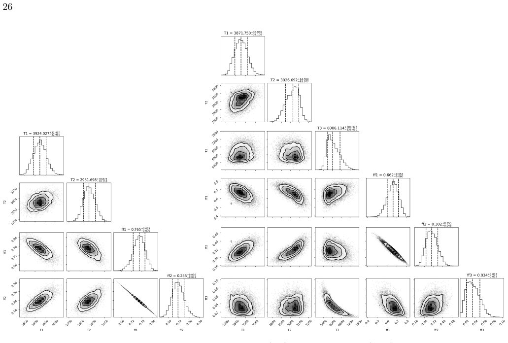
Garcia, L. J., Moran, S. E., Rackham, B. V., et al. 2022, A&A, 665, A19, doi: 10.1051/0004-6361/202142603 26 Figure 14.Corner plots for the 2-temperature (left) and 3-temperature (right) SED fits. Garc´ ıa Soto, A., Duvvuri, G. M., Newton, E. R., et al. 2025, ApJ, 982, 98, doi: 10.3847/1538-4357/adb615
-
[27]
Gelman, A., & Rubin, D. B. 1992, Statistical Science, 7, 457, doi: 10.1214/ss/1177011136
-
[28]
Gilbert, E. A., Barclay, T., Quintana, E. V., et al. 2022, AJ, 163, 147, doi: 10.3847/1538-3881/ac23ca
-
[29]
Ginzburg, S., Schlichting, H. E., & Sari, R. 2016, ApJ, 825, 29, doi: 10.3847/0004-637X/825/1/29
-
[30]
Gupta, A., & Schlichting, H. E. 2019, MNRAS, 487, 24, doi: 10.1093/mnras/stz1230
-
[31]
Schlichting, H. E. 2024, MNRAS, 531, 3698, doi: 10.1093/mnras/stae1376
-
[32]
The No-U-Turn Sampler: Adaptively Setting Path Lengths in Hamiltonian Monte Carlo
Hoffman, M. D., & Gelman, A. 2011, arXiv e-prints, arXiv:1111.4246, doi: 10.48550/arXiv.1111.4246
work page internal anchor Pith review Pith/arXiv arXiv doi:10.48550/arxiv.1111.4246 2011
-
[33]
1986, PASP, 98, 609, doi: 10.1086/131801
Horne, K. 1986, PASP, 98, 609, doi: 10.1086/131801
-
[34]
Howard, W. S., & MacGregor, M. A. 2022, ApJ, 926, 204, doi: 10.3847/1538-4357/ac426e
-
[35]
Howard, W. S., Kowalski, A. F., Flagg, L., et al. 2023, ApJ, 959, 64, doi: 10.3847/1538-4357/acfe75
-
[36]
Hunter, J. D. 2007, Computing in Science & Engineering, 9, 90, doi: 10.1109/MCSE.2007.55
-
[37]
Iyer, A. R., & Line, M. R. 2020, ApJ, 889, 78, doi: 10.3847/1538-4357/ab612e
-
[38]
Kalas, P., Liu, M. C., & Matthews, B. C. 2004, Science, 303, 1990, doi: 10.1126/science.1093420
-
[39]
Keers, R. E., Shapiro, A. I., Kostogryz, N. M., et al. 2024, ApJL, 977, L7, doi: 10.3847/2041-8213/ad8b51
-
[40]
Kempton, E. M.-R., Zhang, M., Bean, J. L., et al. 2023, Nature, 620, 67, doi: 10.1038/s41586-023-06159-5
-
[41]
Kitzmann, D., Stock, J. W., & Patzer, A. B. C. 2024, MNRAS, 527, 7263, doi: 10.1093/mnras/stad3515
-
[42]
2021, MNRAS, 502, 188, doi: 10.1093/mnras/staa3702
Klein, B., Donati, J.-F., Moutou, C., et al. 2021, MNRAS, 502, 188, doi: 10.1093/mnras/staa3702
-
[43]
A., Dragomir, D., Kreidberg, L., et al
Knutson, H. A., Dragomir, D., Kreidberg, L., et al. 2014, ApJ, 794, 155, doi: 10.1088/0004-637X/794/2/155
-
[44]
Kostogryz, N. M., Witzke, V., Shapiro, A. I., et al. 2022, A&A, 666, A60, doi: 10.1051/0004-6361/202243722
-
[45]
R., & Bushouse, H
Kuntschner, H., K¨ ummel, M., Walsh, J. R., & Bushouse, H. 2011,, ST-ECF Instrument Science Report WFC3-2011-05, 13 pages
2011
-
[46]
Kurucz, R. L. 1993, Physica Scripta Volume T, 47, 110, doi: 10.1088/0031-8949/1993/T47/017
-
[47]
2020, The Journal of Open Source Software, 5, 2281, doi: 10.21105/joss.02281
Laginja, I., & Wakeford, H. 2020, The Journal of Open Source Software, 5, 2281, doi: 10.21105/joss.02281
-
[48]
2023, ApJL, 955, L22, doi: 10.3847/2041-8213/acf7c4 27
Lim, O., Benneke, B., Doyon, R., et al. 2023, ApJL, 955, L22, doi: 10.3847/2041-8213/acf7c4 27
-
[49]
Livingston, J. H., Petigura, E. A., David, T. J., et al. 2026, Nature, 649, 310, doi: 10.1038/s41586-025-09840-z
-
[50]
J., Miguel, Y., Tsai, S.-M., et al
Louca, A. J., Miguel, Y., Tsai, S.-M., et al. 2023, MNRAS, 521, 3333, doi: 10.1093/mnras/stac1220
-
[51]
2022, Science, 377, 1211, doi: 10.1126/science.abl7164
Luque, R., & Pall´ e, E. 2022, Science, 377, 1211, doi: 10.1126/science.abl7164
-
[52]
Madhusudhan, N., Sarkar, S., Constantinou, S., et al. 2023, ApJL, 956, L13, doi: 10.3847/2041-8213/acf577 Mallorqu´ ın, M., B´ ejar, V. J. S., Lodieu, N., et al. 2024, A&A, 689, A132, doi: 10.1051/0004-6361/202450047
-
[53]
Mamajek, E. E., & Bell, C. P. M. 2014, MNRAS, 445, 2169, doi: 10.1093/mnras/stu1894
-
[54]
Martioli, E., H´ ebrard, G., Correia, A. C. M., Laskar, J., & Lecavelier des Etangs, A. 2021, A&A, 649, A177, doi: 10.1051/0004-6361/202040235
-
[55]
2011, Python for High Performance and Scientific Computing, 14
McKinney, W. 2011, Python for High Performance and Scientific Computing, 14
2011
-
[56]
2023, MNRAS, 525, 5168, doi: 10.1093/mnras/stad2557
Modi, A., Estrela, R., & Valio, A. 2023, MNRAS, 525, 5168, doi: 10.1093/mnras/stad2557
-
[57]
Moran, S. E., Stevenson, K. B., Sing, D. K., et al. 2023, ApJL, 948, L11, doi: 10.3847/2041-8213/accb9c
-
[58]
Morris, B. M. 2020a, The Journal of Open Source Software, 5, 2103, doi: 10.21105/joss.02103
-
[59]
Morris, B. M. 2020b, The Astrophysical Journal, 893, 67, doi: 10.3847/1538-4357/ab79a0
-
[60]
Narrett, I. S., Rackham, B. V., & de Wit, J. 2024, AJ, 167, 107, doi: 10.3847/1538-3881/ad1f6c
-
[61]
Nixon, M. C., Somers, R. S., Savel, A. B., et al. 2025, ApJ, 995, 95, doi: 10.3847/1538-4357/ae17c8
-
[62]
Owen, J. E. 2019, Annual Review of Earth and Planetary Sciences, 47, 67, doi: 10.1146/annurev-earth-053018-060246
-
[63]
Owen, J. E., & Jackson, A. P. 2012, MNRAS, 425, 2931, doi: 10.1111/j.1365-2966.2012.21481.x
-
[64]
Owen, J. E., & Wu, Y. 2013, ApJ, 775, 105, doi: 10.1088/0004-637X/775/2/105
work page internal anchor Pith review doi:10.1088/0004-637x/775/2/105 2013
-
[65]
Owen, J. E., & Wu, Y. 2016, ApJ, 817, 107, doi: 10.3847/0004-637X/817/2/107
-
[66]
Owen, J. E., & Wu, Y. 2017, ApJ, 847, 29, doi: 10.3847/1538-4357/aa890a
-
[67]
R., Barclay, T., Youngblood, A., et al
Paudel, R. R., Barclay, T., Youngblood, A., et al. 2024, ApJ, 971, 24, doi: 10.3847/1538-4357/ad487d
-
[68]
Composable Effects for Flexible and Accelerated Probabilistic Programming in NumPyro
Phan, D., Pradhan, N., & Jankowiak, M. 2019, arXiv preprint arXiv:1912.11554
work page internal anchor Pith review Pith/arXiv arXiv 2019
-
[69]
2020, Nature, 582, 497, doi: 10.1038/s41586-020-2400-z
Plavchan, P., Barclay, T., Gagn´ e, J., et al. 2020, Nature, 582, 497, doi: 10.1038/s41586-020-2400-z
-
[70]
Rackham, B. V., Apai, D., & Giampapa, M. S. 2018, ApJ, 853, 122, doi: 10.3847/1538-4357/aaa08c
-
[71]
Rackham, B. V., Apai, D., & Giampapa, M. S. 2019, AJ, 157, 96, doi: 10.3847/1538-3881/aaf892
-
[72]
Rackham, B. V., & de Wit, J. 2024, AJ, 168, 82, doi: 10.3847/1538-3881/ad5833
-
[73]
Rockcliffe, K. E., Newton, E. R., Youngblood, A., et al. 2023, AJ, 166, 77, doi: 10.3847/1538-3881/ace536
-
[74]
Seager, S., & Shapiro, A. I. 2024, ApJ, 970, 155, doi: 10.3847/1538-4357/ad509a
-
[75]
Sing, D. K. 2018, arXiv e-prints, arXiv:1804.07357, doi: 10.48550/arXiv.1804.07357
work page internal anchor Pith review Pith/arXiv arXiv doi:10.48550/arxiv.1804.07357 2018
-
[76]
Smitha, H. N., Shapiro, A. I., Witzke, V., et al. 2025, ApJL, 978, L13, doi: 10.3847/2041-8213/ad9aaa
-
[77]
Solanki, S. K. 2003, A&A Rv, 11, 153, doi: 10.1007/s00159-003-0018-4
-
[78]
Steinmeyer, M.-L., Dorn, C., Werlen, A., & Grimm, S. L. 2026, ApJ, 1001, 36, doi: 10.3847/1538-4357/ae4c47
-
[79]
Stevenson, K. B., Bean, J. L., Fabrycky, D., & Kreidberg, L. 2014, ApJ, 796, 32, doi: 10.1088/0004-637X/796/1/32
-
[80]
Stock, J. W., Kitzmann, D., & Patzer, A. B. C. 2022, MNRAS, 517, 4070, doi: 10.1093/mnras/stac2623
discussion (0)
Sign in with ORCID, Apple, or X to comment. Anyone can read and Pith papers without signing in.