CoFL: Continuous Flow Fields for Language-Conditioned Navigation
Pith reviewed 2026-05-15 17:14 UTC · model grok-4.3
The pith
CoFL learns continuous flow fields from bird's-eye views and language instructions to navigate unseen scenes more precisely than trajectory predictors or modular planners.
A machine-rendered reading of the paper's core claim, the machinery that carries it, and where it could break.
Core claim
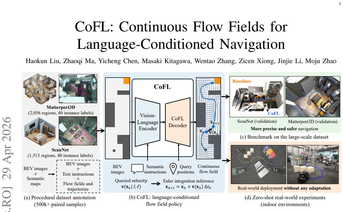
CoFL reformulates language-conditioned navigation as workspace-conditioned field learning: it maps any bird's-eye view location to a motion vector conditioned on the language instruction, so that each scene-instruction annotation supplies dense supervision instead of a single start-conditioned rollout. Trajectories are recovered from arbitrary starts by integrating the predicted field, enabling simple real-time closed-loop control and recovery from deviations.
What carries the argument
The continuous flow field, which assigns a local motion vector to every point in the bird's-eye view workspace conditioned on the language instruction and is used to generate paths by numerical integration.
If this is right
- Each scene-instruction annotation now supplies dense spatial supervision rather than a single trajectory, increasing training signal per example.
- Numerical integration of the field from any start enables closed-loop recovery without retraining.
- The policy achieves higher navigation precision and safety than modular VLM planners or start-conditioned trajectory generators on unseen scenes.
- Real-time inference is preserved while supporting zero-shot transfer to physical robot deployments.
- The same field representation works across multiple room layouts without scene-specific retraining.
Where Pith is reading between the lines
- The method could lower annotation costs by replacing manual trajectory labels with procedural flow fields from existing semantic maps.
- Similar field-based representations might apply to other robotics tasks such as manipulation or multi-agent coordination where continuous guidance is useful.
- Online fusion with live semantic mapping could allow the flow field to adapt to dynamic changes without full retraining.
- The integration-based rollout naturally provides a mechanism for uncertainty-aware planning by sampling multiple paths through the field.
Load-bearing premise
Flow fields procedurally derived from semantic maps in simulation supply accurate and generalizable supervision for arbitrary language instructions when the system is deployed in real physical environments.
What would settle it
A controlled real-world trial in which the robot, following the integrated flow field, deviates from the language-specified goal or collides in a novel layout where the simulation-derived semantic map no longer matches physical geometry.
Figures


read the original abstract
Existing language-conditioned navigation systems typically rely on modular pipelines or trajectory generators, but the latter use each scene--instruction annotation mainly to supervise one start-conditioned rollout. To address these limitations, we present CoFL, an end-to-end policy that maps a bird's-eye view (BEV) observation and a language instruction to a continuous flow field for navigation. CoFL reformulates navigation as workspace-conditioned field learning rather than start-conditioned trajectory prediction: it learns local motion vectors at arbitrary BEV locations, turning each scene--instruction annotation into dense spatial control supervision. Trajectories are generated from any start by numerical integration of the predicted field, enabling simple real-time rollout and closed-loop recovery. To enable large-scale training and evaluation, we build a dataset of over 500k BEV image--instruction pairs, each procedurally annotated with a flow field and a trajectory derived from semantic maps built on Matterport3D and ScanNet. Evaluating on strictly unseen scenes, CoFL significantly outperforms modular Vision-Language Model (VLM)-based planners and trajectory generation policies in both navigation precision and safety, while maintaining real-time inference. Finally, we deploy CoFL zero-shot in real-world experiments with BEV observations across multiple layouts, maintaining feasible closed-loop control and a high success rate.
Editorial analysis
A structured set of objections, weighed in public.
Referee Report
Summary. The manuscript introduces CoFL, an end-to-end policy that maps bird's-eye-view (BEV) observations and language instructions to continuous flow fields for navigation. It reformulates the problem as learning local motion vectors at arbitrary BEV locations rather than start-conditioned trajectories, using numerical integration to generate paths. The approach is trained on over 500k procedurally generated BEV-instruction pairs derived from semantic maps on Matterport3D and ScanNet. The central claim is that CoFL significantly outperforms modular VLM-based planners and trajectory-generation policies on strictly unseen scenes in navigation precision and safety, supports real-time inference, and succeeds in zero-shot real-world closed-loop deployment.
Significance. If the performance claims hold under detailed scrutiny, the reformulation to dense flow-field supervision could improve generalization and closed-loop recovery compared to sparse trajectory supervision. The scale of the procedurally generated dataset is a notable strength for training. However, the absence of quantitative metrics, error bars, or ablation details in the abstract limits assessment of practical impact on embodied navigation.
major comments (3)
- [Abstract] Abstract: the claim of significant outperformance on unseen scenes in precision and safety is stated without any quantitative metrics, success rates, error bars, baseline implementations, or ablation studies, preventing verification of the central empirical result.
- [Real-world experiments] Real-world experiments section: the zero-shot deployment reports feasible closed-loop control and high success rate across layouts, but provides no quantitative metrics, description of the real BEV pipeline, or handling of sensor noise and semantic labeling errors, leaving the sim-to-real transfer assumption untested.
- [Methods] Methods: the procedural flow fields are derived from clean simulation semantic maps to provide dense supervision, yet no ablation on perception noise, labeling errors, or BEV quality is reported; this directly bears on whether the learned field remains accurate for arbitrary instructions under real-world conditions.
minor comments (1)
- [Abstract] Abstract: the phrase 'workspace-conditioned field learning' is introduced without a brief definition or pointer to related field-based navigation literature, which could aid readability.
Simulated Author's Rebuttal
We thank the referee for the constructive comments. We address each major point below and have revised the manuscript to strengthen the empirical presentation and robustness analysis.
read point-by-point responses
-
Referee: [Abstract] Abstract: the claim of significant outperformance on unseen scenes in precision and safety is stated without any quantitative metrics, success rates, error bars, baseline implementations, or ablation studies, preventing verification of the central empirical result.
Authors: We agree that the abstract would be strengthened by including key quantitative results. In the revised manuscript we will add specific metrics such as success rates on unseen scenes, navigation error reductions relative to baselines, and error bars to support the claims of outperformance in precision and safety. revision: yes
-
Referee: [Real-world experiments] Real-world experiments section: the zero-shot deployment reports feasible closed-loop control and high success rate across layouts, but provides no quantitative metrics, description of the real BEV pipeline, or handling of sensor noise and semantic labeling errors, leaving the sim-to-real transfer assumption untested.
Authors: We acknowledge the need for more detail. We will expand the real-world section to report quantitative success rates and failure statistics across trials, provide a description of the real BEV observation pipeline, and discuss mitigation strategies for sensor noise and semantic labeling errors to better substantiate the sim-to-real transfer. revision: yes
-
Referee: [Methods] Methods: the procedural flow fields are derived from clean simulation semantic maps to provide dense supervision, yet no ablation on perception noise, labeling errors, or BEV quality is reported; this directly bears on whether the learned field remains accurate for arbitrary instructions under real-world conditions.
Authors: This is a valid concern. We will add an ablation study in the revised manuscript that introduces controlled perception noise and labeling errors into the BEV inputs and reports the resulting degradation in flow-field accuracy and downstream navigation performance. revision: yes
Circularity Check
No circularity: empirical evaluation on held-out scenes
full rationale
The paper's core claim is an empirical performance comparison: a policy trained on procedurally generated flow-field supervision from semantic maps is evaluated on strictly unseen scenes and real-world zero-shot deployment. The flow fields serve as training targets derived from external semantic maps (Matterport3D/ScanNet), not as a self-referential definition or fitted parameter renamed as prediction. No equations reduce the output trajectory to the input by construction, no load-bearing self-citations justify uniqueness, and no ansatz is smuggled via prior work. The derivation chain is a standard supervised learning pipeline whose success is measured by external benchmarks rather than internal equivalence.
Axiom & Free-Parameter Ledger
free parameters (1)
- Neural network weights
axioms (1)
- domain assumption BEV observations combined with language instructions contain sufficient information to define valid navigation flow fields
invented entities (1)
-
Continuous flow field
no independent evidence
Reference graph
Works this paper leans on
-
[1]
RT-1: Robotics Transformer for Real-World Control at Scale,
A. Brohanet al., “RT-1: Robotics Transformer for Real-World Control at Scale,” inProceedings of Robotics: Science and Systems, Daegu, Republic of Korea, July 2023
work page 2023
-
[2]
RT-2: Vision-language-action models transfer web knowledge to robotic control,
B. Zitkovichet al., “RT-2: Vision-language-action models transfer web knowledge to robotic control,” in7th Annual Conference on Robot Learning, 2023
work page 2023
-
[3]
OpenVLA: An open-source vision-language-action model,
M. J. Kimet al., “OpenVLA: An open-source vision-language-action model,” in8th Annual Conference on Robot Learning, 2024
work page 2024
-
[4]
Diffusion policy: Visuomotor policy learning via action diffusion,
C. Chiet al., “Diffusion policy: Visuomotor policy learning via action diffusion,”The International Journal of Robotics Research, vol. 44, no. 10-11, pp. 1684–1704, 2025
work page 2025
-
[5]
π 0: A Vision-Language-Action Flow Model for General Robot Control,
K. Blacket al., “π 0: A Vision-Language-Action Flow Model for General Robot Control,” inProceedings of Robotics: Science and Systems, LosAngeles, CA, USA, June 2025
work page 2025
-
[6]
π 0.5: a vision-language-action model with open-world general- ization,
——, “π 0.5: a vision-language-action model with open-world general- ization,” in9th Annual Conference on Robot Learning, 2025
work page 2025
-
[7]
Matterport3d: Learning from rgb-d data in indoor environments,
A. Changet al., “Matterport3d: Learning from rgb-d data in indoor environments,” in2017 International Conference on 3D Vision (3DV). IEEE Computer Society, 2017, pp. 667–676
work page 2017
-
[8]
Scannet: Richly-annotated 3d reconstructions of indoor scenes,
A. Dai, A. X. Chang, M. Savva, M. Halber, T. Funkhouser, and M. Nießner, “Scannet: Richly-annotated 3d reconstructions of indoor scenes,” inProceedings of the IEEE conference on computer vision and pattern recognition, 2017, pp. 5828–5839
work page 2017
-
[9]
Adaptive teams of autonomous aerial and ground robots for situational awareness,
M. A. Hsiehet al., “Adaptive teams of autonomous aerial and ground robots for situational awareness,”Journal of field robotics, vol. 24, no. 11-12, pp. 991–1014, 2007
work page 2007
-
[10]
Bird’s eye view: Cooperative exploration by ugv and uav,
S. Hood, K. Benson, P. Hamod, D. Madison, J. M. O’Kane, and I. Rekleitis, “Bird’s eye view: Cooperative exploration by ugv and uav,” in2017 International Conference on Unmanned Aircraft Systems (ICUAS). IEEE, 2017, pp. 247–255
work page 2017
-
[11]
Graph-based subterranean exploration path planning using aerial and legged robots,
T. Dang, M. Tranzatto, S. Khattak, F. Mascarich, K. Alexis, and M. Hutter, “Graph-based subterranean exploration path planning using aerial and legged robots,”Journal of Field Robotics, vol. 37, no. 8, pp. 1363–1388, 2020
work page 2020
-
[12]
Collaborative multi-robot search and rescue: Planning, coordination, perception, and active vision,
J. P. Queraltaet al., “Collaborative multi-robot search and rescue: Planning, coordination, perception, and active vision,”Ieee Access, vol. 8, pp. 191 617–191 643, 2020
work page 2020
-
[13]
Deploying foundation model-enabled air and ground robots in the field: Challenges and opportunities,
Z. Ravichandranet al., “Deploying foundation model-enabled air and ground robots in the field: Challenges and opportunities,”arXiv preprint arXiv:2505.09477, 2025
-
[14]
H. Liuet al., “Hierarchical language models for semantic navigation and manipulation in an aerial-ground robotic system,”Advanced Intelligent Systems, p. e202500640, 2025
work page 2025
-
[15]
Lift, splat, shoot: Encoding images from arbitrary camera rigs by implicitly unprojecting to 3d,
J. Philion and S. Fidler, “Lift, splat, shoot: Encoding images from arbitrary camera rigs by implicitly unprojecting to 3d,” inEuropean conference on computer vision. Springer, 2020, pp. 194–210
work page 2020
-
[16]
Z. Liet al., “Bevformer: learning bird’s-eye-view representation from lidar-camera via spatiotemporal transformers,”IEEE Transactions on Pattern Analysis and Machine Intelligence, 2024
work page 2024
-
[17]
P. Andersonet al., “Vision-and-language navigation: Interpreting visually-grounded navigation instructions in real environments,” in Proceedings of the IEEE conference on computer vision and pattern recognition, 2018, pp. 3674–3683
work page 2018
-
[18]
Do as i can, not as i say: Grounding language in robotic affordances,
B. Ichteret al., “Do as i can, not as i say: Grounding language in robotic affordances,” in6th Annual Conference on Robot Learning, 2022
work page 2022
-
[19]
LM-nav: Robotic navigation with large pre-trained models of language, vision, and action,
D. Shah, B. Osi ´nski, brian ichter, and S. Levine, “LM-nav: Robotic navigation with large pre-trained models of language, vision, and action,” in6th Annual Conference on Robot Learning, 2022
work page 2022
-
[20]
Cows on pasture: Baselines and benchmarks for language-driven zero-shot object navigation,
S. Y . Gadre, M. Wortsman, G. Ilharco, L. Schmidt, and S. Song, “Cows on pasture: Baselines and benchmarks for language-driven zero-shot object navigation,” inProceedings of the IEEE/CVF Conference on Computer Vision and Pattern Recognition, 2023, pp. 23 171–23 181
work page 2023
-
[21]
Code as policies: Language model programs for embodied control,
J. Lianget al., “Code as policies: Language model programs for embodied control,” in2023 IEEE International Conference on Robotics and Automation (ICRA), 2023, pp. 9493–9500
work page 2023
-
[22]
Mapgpt: Map-guided prompting with adaptive path planning for vision-and- language navigation,
J. Chen, B. Lin, R. Xu, Z. Chai, X. Liang, and K.-Y . Wong, “Mapgpt: Map-guided prompting with adaptive path planning for vision-and- language navigation,” inProceedings of the 62nd Annual Meeting of the Association for Computational Linguistics (Volume 1: Long Papers), 2024, pp. 9796–9810
work page 2024
-
[23]
Enhancing the llm-based robot manipulation through human-robot collaboration,
H. Liuet al., “Enhancing the llm-based robot manipulation through human-robot collaboration,”IEEE Robotics and Automation Letters, vol. 9, no. 8, pp. 6904–6911, 2024
work page 2024
-
[24]
Palm-e: An embodied multimodal language model,
D. Driesset al., “Palm-e: An embodied multimodal language model,” in International Conference on Machine Learning, 2023, pp. 8469–8488
work page 2023
-
[25]
Denoising diffusion probabilistic models,
J. Ho, A. Jain, and P. Abbeel, “Denoising diffusion probabilistic models,” Advances in neural information processing systems, vol. 33, pp. 6840– 6851, 2020
work page 2020
-
[26]
Training diffu- sion models with reinforcement learning,
K. Black, M. Janner, Y . Du, I. Kostrikov, and S. Levine, “Training diffu- sion models with reinforcement learning,” inThe Twelfth International Conference on Learning Representations, 2024
work page 2024
-
[27]
Y . Song, P. Dhariwal, M. Chen, and I. Sutskever, “Consistency models,” inInternational Conference on Machine Learning. PMLR, 2023, pp. 32 211–32 252
work page 2023
-
[28]
Two-steps diffusion policy for robotic manipulation via genetic denoising,
M. Cl ´ementeet al., “Two-steps diffusion policy for robotic manipulation via genetic denoising,” inThe Thirty-ninth Annual Conference on Neural Information Processing Systems, 2025
work page 2025
-
[29]
Flow matching for generative modeling,
Y . Lipman, R. T. Chen, H. Ben-Hamu, M. Nickel, and M. Le, “Flow matching for generative modeling,” in11th International Conference on Learning Representations, ICLR 2023, 2023
work page 2023
-
[30]
Flow straight and fast: Learning to generate and transfer data with rectified flow,
X. Liu, C. Gong, and Q. Liu, “Flow straight and fast: Learning to generate and transfer data with rectified flow,” inThe Eleventh International Conference on Learning Representations, 2023
work page 2023
-
[31]
$\pi^{*}_{0.6}$: a VLA That Learns From Experience
P. Intelligenceet al., “π ∗ 0.6: a vla that learns from experience,”arXiv preprint arXiv:2511.14759, 2025
work page internal anchor Pith review Pith/arXiv arXiv 2025
-
[32]
Real-time obstacle avoidance for manipulators and mobile robots,
O. Khatib, “Real-time obstacle avoidance for manipulators and mobile robots,”The international journal of robotics research, vol. 5, no. 1, pp. 90–98, 1986
work page 1986
-
[33]
Neural potential field for obstacle-aware local motion planning,
M. Alhaddad, K. Mironov, A. Staroverov, and A. Panov, “Neural potential field for obstacle-aware local motion planning,” in2024 IEEE International Conference on Robotics and Automation (ICRA), 2024, pp. 9313–9320
work page 2024
-
[34]
Sigmoid loss for language image pre-training,
X. Zhai, B. Mustafa, A. Kolesnikov, and L. Beyer, “Sigmoid loss for language image pre-training,” inProceedings of the IEEE/CVF international conference on computer vision, 2023, pp. 11 975–11 986
work page 2023
-
[35]
M. Tschannenet al., “Siglip 2: Multilingual vision-language encoders with improved semantic understanding, localization, and dense features,” arXiv preprint arXiv:2502.14786, 2025
work page internal anchor Pith review Pith/arXiv arXiv 2025
-
[36]
A. Vaswaniet al., “Attention is all you need,” inAdvances in Neural Information Processing Systems, I. Guyonet al., Eds., vol. 30. Curran Associates, Inc., 2017
work page 2017
-
[37]
End-to-end object detection with transformers,
N. Carion, F. Massa, G. Synnaeve, N. Usunier, A. Kirillov, and S. Zagoruyko, “End-to-end object detection with transformers,” in European conference on computer vision. Springer, 2020, pp. 213– 229
work page 2020
-
[38]
Fourier features let networks learn high frequency functions in low dimensional domains,
M. Tanciket al., “Fourier features let networks learn high frequency functions in low dimensional domains,”Advances in neural information processing systems, vol. 33, pp. 7537–7547, 2020
work page 2020
-
[39]
A note on two problems in connexion with graphs,
E. Dijkstra, “A note on two problems in connexion with graphs,” Numerische Mathematik, vol. 1, pp. 269–271, 1959
work page 1959
-
[40]
D. Goetting, H. G. Singh, and A. Loquercio, “End-to-end naviga- tion with vision-language models: Transforming spatial reasoning into question-answering,” inProceedings of the International Conference on Neuro-symbolic Systems, ser. Proceedings of Machine Learning Research, G. Pappas, P. Ravikumar, and S. A. Seshia, Eds., vol. 288. PMLR, 28–30 May 2025, pp. 22–35
work page 2025
-
[41]
Film: Visual reasoning with a general conditioning layer,
E. Perez, F. Strub, H. de Vries, V . Dumoulin, and A. Courville, “Film: Visual reasoning with a general conditioning layer,”Proceedings of the AAAI Conference on Artificial Intelligence, vol. 32, no. 1, Apr. 2018. SUPPLEMENTARYMATERIAL For completeness, we provide additional appendix materials in the supplementary document. The supplementary material incl...
work page 2018
-
[42]
Free/Obstacle Masks:Given the semantic mapS,EX- TRACTFREEconstructs a binary free-space maskM free ∈ {0,1} H×W using the predefined dataset-specific label map- pingR. Pixels whose semantic labels belong to the free set are marked asM free=1, and we defineM obs =¬M free
-
[43]
Goal Sources:COMPUTEGOALreturns goal source pixelsp g from the target instance specified byℓ target, typically as a thin boundary band adjacent to the target in free space. Whenℓ target contains directional modifiers, such as left/right or front/back, the goal source is restricted to the corresponding side of the target boundary in the BEV coordinate fram...
-
[44]
Distance-to-obstacle Transform:DTOcomputes the Euclidean distance transformD free over free spaceM free = 1, whereD free(p)is the distance (in pixels) from a free pixelp to the nearest obstacle pixel
-
[45]
Intuitively, this increases costs near obstacles and encourages paths with larger clearance
Safety-aware Cost Map:COSTMAPconvertsD free into a traversal cost mapC cost ≥1by applying a truncated linear penalty within a safety band of radiusρ safe: Ccost(p) = 1 +λ safe [ρsafe −D free(p)]+,(24) where[z] + = max(0, z). Intuitively, this increases costs near obstacles and encourages paths with larger clearance
-
[46]
We treat each free pixel as a graph node
Cost-weighted Geodesic and Predecessor Map: GEODESICruns the Dijkstra [39] on an 8-connected pixel grid, restricted to free cells (M free=1). We treat each free pixel as a graph node. For any two neighboring pixelspand q(axial/diagonal neighbors), we assign an edge cost w(p,q) = 1 2 Ccost(p) +C cost(q) ∥p−q∥ 2,(25) where∥p−q∥ 2 ∈ {1, √ 2}for axial/diagona...
-
[47]
Pixel Distance-to-go Along the Predecessor Tree:PIX- ELLENGTHFROMPREDcomputesD pix g (p), defined as the geometric remaining path length (in pixels) when repeatedly following the predecessor pointers frompto a goal. Equiva- lently, it is the accumulated step length along the predecessor chain: Dpix g (p) = K(p)−1X k=0 pk −p k+1 2, p0 =p,p k+1 = pred(pk),(...
-
[48]
Potential Construction:We form a piecewise potential Φfollowing Algorithm 1: Φ(p) = ( wg Dw g (p),M free(p) = 1, wobs Dobs(p) +b obs,M obs(p) = 1. (27) We setw obs ≫w g and chooseb obs = maxp:M free(p)=1 wgDw g (p)such that the obstacle-side potentials dominate around the interface, avoiding discrete gradients that point into obstacles
-
[49]
Direction and Magnitude:We smoothΦwith a Gaussian filter and compute spatial derivatives using Sobel operators. The unit direction field is u(p) = −∇Φ(p) ∥∇Φ(p)∥2 +ϵ .(28) In free space, we scale the magnitude by the pixel distance- to-go and convert it to normalized coordinates:V ∗(p) = ux(p)·D pix g (p)/W, u y(p)·D pix g (p)/H ,forM free(p) = 1. Inside ...
-
[50]
Reachable Free Space and Start Sampling:Although Mfree marks all non-obstacle pixels, some free regions may be disconnected from the goal sources (e.g., being fully enclosed by obstacles). Therefore,SAMPLESTARTsamples the start pixelp 0 only from the reachable subset, defined by a finite distance-to-go:D pix g (p0)<∞. The sampled start is further required...
-
[51]
Backtracking and Resampling:Givenp 0,BACK- TRACKPREDbacktracks predecessorsp k+1 = pred(pk)until reaching a goal source to obtain a polylineτ raw.RESAMPLE then resamplesτ raw by arc length to a fixed number of way- points to obtainτ ∗, which is stored in normalized coordinates (px/W, p y/H). APPENDIXB DETAILS OFEVALUATIONMETRICS ANDPROTOCOL We describe th...
-
[52]
Final Goal Error (FGE):Letx end ∈[0,1] 2 be the endpoint of the annotated trajectoryτ ∗. FGE is the Euclidean distance between the final resampled point and the endpoint: FGE(¯τ) =∥¯ xK−1 −x end∥2 .(30)
-
[53]
Collision Rate (CR):CR is a binary indicator of whether the resampled predicted trajectory ever enters an obstacle cell: CR(¯τ) =I h ∃j:M obs[py(¯ xj), px(¯ xj)] = 1 i .(31) The benchmark reports the mean ofCR(τ)across episodes
-
[54]
Let segment vectors be∆ j =¯ xj+1 −¯ xj
Curvature-based Smoothness (Curv):Curvature is the mean absolute change in heading angle between consecutive segments of the resampled predicted trajectory. Let segment vectors be∆ j =¯ xj+1 −¯ xj. We discard degenerate segments with∥∆ j∥2 ≤ϵand compute headings ψj = atan2(∆(v) j ,∆ (u) j ).(32) Curv is then Curv(¯τ) = 1 M−1 M−2X j=0 |WrapToPi(ψj+1 −ψ j)|...
-
[55]
Flow Field Metrics Flow field metrics are evaluated on the exact grid of the annotated flow
Path Length Ratio (PLR):Let the path length of a resampled trajectory be L(¯τ) = K−2X j=0 ∥¯ xj+1 −¯ xj∥2 .(34) PLR is defined as the ratio between predicted and annotated trajectory lengths: PLR(¯τ) = L(¯τ) L(τ ∗) .(35) C. Flow Field Metrics Flow field metrics are evaluated on the exact grid of the annotated flow. Let the annotated flow have a spatial re...
-
[56]
AE is the mean of{∆ϕ n}over all evaluated points
Angular Error (AE):We compute the clipped cosine similarity cn = clip ˆVn ∥ˆVn∥2 +ϵ · Vn ∗ ∥Vn ∗∥2 +ϵ ,−1,1 ! ,(36) and define the per-point angular error as∆ϕ n = arccos(cn)· 180 π (degrees). AE is the mean of{∆ϕ n}over all evaluated points
-
[57]
All baselines operate on the same BEV observationI, language instruction ℓ, and start positionx 0
Magnitude Error (ME):Magnitude error is ME = 1 N NX n=1 ∥ˆVn∥2 − ∥Vn ∗∥2 .(37) APPENDIXC DETAILS OFBASELINEIMPLEMENTATIONS This appendix describes baseline formulations and imple- mentation details as a supplement for §V-A. All baselines operate on the same BEV observationI, language instruction ℓ, and start positionx 0. Learned baselines use the same fro...
-
[58]
notes" using short ASCII words (e.g.,
Prompt:We use the following system prompt and re- quest a strict JSON response: System prompt for Pure VLM baseline You are a robot navigation policy operating on a TOP-DOWN VIEW (bird’s eye view) and a natural-language instruction. INPUTS 15 - Image: a TOP-DOWN VIEW (bird’s eye view) (RGB-only; no explicit obstacle mask). - Text: (1) Instruction and (2) ...
-
[59]
The VLM is instructed to trust the text start if the visualization is unclear
Query Format:To reduce ambiguity in the start location, we additionally draw a green dot on the input map, while still providing the authoritative start coordinate in text. The VLM is instructed to trust the text start if the visualization is unclear
-
[60]
We set the maximum output budget to 8192 tokens to reduce truncation
Decoding and API Settings:We use Gemini-2.5-Flash with deterministic decoding (temperature= 0, top-p= 1.0) and enforce a JSON-only response format. We set the maximum output budget to 8192 tokens to reduce truncation. If the output is malformed, we retry up to two times
-
[61]
All coordinates are clamped to[0,1]
Output Parsing and Waypoint Normalization:We parse the returned JSON object and extracttargetand trajectory. All coordinates are clamped to[0,1]. If the returned trajectory contains fewer than the required number of waypoints, we interpolate along its arclength to obtain exactlyNwaypoints; if it contains more, we subsample uniformly by index. This post-pr...
-
[62]
VLM Prediction (Target and Obstacles):The VLM outputs a JSON object containing the target object (center and bounding box), a list of obstacle objects (each with a center and bounding box), and an optional start estimate. We use the following system instruction and request JSON-only output: System prompt for VLM in VLM+Planner baseline You are analyzing a...
-
[63]
The TARGET OBJECT (the object the instruction refers to) with its center, bounding box, and direction descriptor (left, right, top, bottom, none)
-
[64]
Other obstacle objects that might block a path, with their centers and bounding boxes
-
[65]
If multiple candidates exist, choose the one you judge to be most consistent with the instruction and overall scene layout. Output ONLY valid JSON. Required keys are exactly: {{"target":{{"name": "object_name", "center": [0.50, 0.70], "bbox": [0.40, 0.60, 0.60, 0.85], "direction": "left/right/top/bottom/none", "confidence": "high/medium/low"}}, "obstacles...
-
[66]
Query Format and Side-of-object Handling:The user query provides the instruction and requests (i) a target and (ii) obstacles. If the instruction specifies approaching a side 16 of an object (e.g.,left of/right of/above/below), we treat the target object’s bounding box as an additional forbidden region and set the navigation goal to a point offset from th...
-
[67]
Decoding and API Settings:We use Gemini-2.5-Flash with deterministic decoding (temperature= 0, top-p= 1.0) and a maximum output budget of 8192 tokens. If the returned JSON is invalid or missing a target bbox/center, we retry up to two times with an explicit JSON-only reminder
-
[68]
Geometric Planning (A*):We rasterize the predicted obstacle bounding boxes into a binary occupancy grid of size G×G(defaultG= 128) and run A* (8-neighborhood) from the provided startx 0 to the derived goal(x g, yg). To enforce a safety margin, we inflate each obstacle by a fixed pixel radius r(10 px in the bbox image space), converted to a normalized marg...
-
[69]
Problem Formulation and Trajectory Parameterization: All DP-family baselines model a trajectory as a length-T sequence of 2D displacements∆X∈R T×2 in normalized image coordinates, withT= 100. Waypoints are recovered by cumulative summation from the initial state: X=x 0 + cumsum(∆X).(39) To improve optimization conditioning and keep the diffusion scale rou...
-
[70]
The encoder outputs a token sequenceC∈R Nv×d that conditions the denoiser
Network Architecture: a) Vision–language encoder (shared):All DP-family baselines reuse the same visual–language encoder as CoFL: SigLIP2-B/16 at224×224, followed by the same cross-modal fusion stack (model dimensiond=768,8heads,4fusion layers). The encoder outputs a token sequenceC∈R Nv×d that conditions the denoiser. b) Conditioning inputs (shared):Both...
-
[71]
Training Objective and Defaults:All DP variants share the same data preprocessing and displacement normalization, but use different training objectives depending on the sampler family. a) DDPM objective (DP-*-DDPM):For stochastic re- verse diffusion, we adopt the standard DDPM noise-prediction parameterization. At a discrete noise leveln∈ {1, . . . , N di...
-
[72]
& ',+ $ % -$ ' **(* 1 Segments n12451020500.1360.1440.1520.1600.168 (a) FGE↓
Inference-Time Sampling:At test time, we sample Gaus- sian noise in displacement space and map it to a displace- ment sequence∆ ˜Xusing the sampler corresponding to each training objective, then recover waypointsXby rescaling and cumulative summation. 18 "& ',+ $ % -$ ' **(* 1 Segments n12451020500.1360.1440.1520.1600.168 (a) FGE↓ "& ',+ (%%$+$(' , 1 Segm...
discussion (0)
Sign in with ORCID, Apple, or X to comment. Anyone can read and Pith papers without signing in.