Model Parameter Reconstruction of Electroweak Phase Transition with TianQin and LISA: Insights from the Dimension-Six Model
Pith reviewed 2026-05-25 07:30 UTC · model grok-4.3
The pith
TianQin and LISA recover the dimension-six operator cutoff scale to sub-percent precision from simulated electroweak phase transition gravitational wave signals.
A machine-rendered reading of the paper's core claim, the machinery that carries it, and where it could break.
Core claim
The central claim is that the mapping from the dimension-six model parameter Λ to observable gravitational wave spectral features permits both TianQin and LISA to reconstruct Λ at sub-percent precision for strong-signal benchmarks, achieved by combining geometric inference on compressed data with subsequent machine-learning steps while treating bubble wall velocity as fixed.
What carries the argument
The direct mapping between the dimension-six operator cutoff Λ and the peak frequency and amplitude of the stochastic gravitational wave spectrum, which serves as the input for Fisher-matrix and PolyChord inference followed by machine-learning reconstruction.
If this is right
- Sub-percent recovery of Λ translates into tight constraints on the new-physics scale that triggers the electroweak phase transition.
- The same data-compression and inference pipeline applies to any new-physics model whose gravitational wave spectrum is governed by a single dominant parameter.
- The 20-30 percent uncertainty on amplitude sets the statistical floor for amplitude measurements with these detectors under the stated noise model.
- Machine-learning post-processing can be inserted after standard geometric inference to improve parameter recovery without altering the underlying likelihood.
Where Pith is reading between the lines
- Extending the pipeline to marginalize over bubble wall velocity would quantify how much the quoted sub-percent precision degrades once that parameter is freed.
- The same reconstruction strategy could be tested on signals from other cosmological phase transitions whose spectra share a similar single-parameter dependence.
- Joint analysis of TianQin and LISA data streams could be examined to determine whether the combined network further tightens the uncertainty on Λ beyond the individual-detector results.
Load-bearing premise
The reconstruction assumes a fixed bubble wall velocity and excludes theoretical uncertainties from the effective potential calculation.
What would settle it
A reconstruction of Λ whose uncertainty exceeds the sub-percent level when the bubble wall velocity is allowed to vary or when theoretical uncertainties in the effective potential are folded into the likelihood would falsify the reported precision.
Figures


read the original abstract
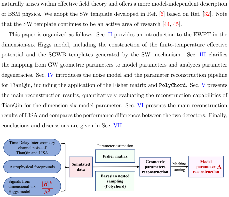
We investigate the capability of TianQin and LISA to reconstruct the model parameters in the Lagrangian of new physics scenarios that can generate an electroweak SFOPT. Taking the dimension-six Higgs operator extension of the Standard Model as a representative scenario for a broad class of new physics models, we establish the mapping between the model parameter $\Lambda$ and the observable spectral features of the stochastic gravitational wave background. We begin by generating simulated data incorporating Time Delay Interferometry channel noise, astrophysical foregrounds, and signals from the dimension-six model. The data are then compressed and optimized, followed by geometric parameter inference using both Fisher matrix analysis and Bayesian nested sampling with PolyChord, which efficiently handles high-dimensional, multimodal posterior distributions. Finally, machine-learning techniques are employed to achieve precise reconstruction of the model parameter $\Lambda$. For benchmark points producing strong signals, parameter reconstruction with both TianQin and LISA yields relative uncertainties of approximately $20$-$30\%$ in the signal amplitude and sub-percent precision in the model parameter $\Lambda$. The sub-percent precision reflects the statistical reconstruction capability of the detectors in an idealized setting: it incorporates the machine-learning inference uncertainty and is established at a fixed bubble wall velocity, while theoretical uncertainties in the effective potential calculation are not included.
Editorial analysis
A structured set of objections, weighed in public.
Referee Report
Summary. The manuscript investigates the reconstruction of the dimension-six model parameter Λ (which controls the strength of the electroweak first-order phase transition) from simulated stochastic gravitational-wave backgrounds observable by TianQin and LISA. Simulated data include TDI channel noise and astrophysical foregrounds; inference combines Fisher-matrix analysis, Bayesian nested sampling via PolyChord, and machine-learning techniques. For benchmark points with strong signals the authors report 20–30 % relative uncertainty on signal amplitude and sub-percent statistical precision on Λ, explicitly qualified as holding at fixed bubble-wall velocity and without theoretical uncertainties in the effective potential.
Significance. If the reported sub-percent precision on Λ survives marginalization over bubble-wall velocity and inclusion of effective-potential uncertainties, the work would provide a concrete demonstration that space-based interferometers can extract new-physics parameters from phase-transition gravitational waves. The use of PolyChord for multimodal posteriors and the explicit mapping from Lagrangian parameter to spectral features are positive technical contributions.
major comments (1)
- [Abstract] Abstract (final sentence) and the reconstruction pipeline description: the headline sub-percent uncertainty on Λ is obtained only after fixing the bubble-wall velocity v_w and omitting theoretical uncertainties in the effective potential. Both choices are known to rescale the predicted GW spectrum by O(1) factors in the dimension-six model; without a sensitivity scan or marginalization over v_w or potential parameters, the quoted precision cannot be interpreted as a realistic detector capability. This assumption is load-bearing for the central claim.
minor comments (2)
- The mapping between Λ and the peak frequency/amplitude of the GW spectrum should be shown explicitly (perhaps as an equation or figure) rather than stated qualitatively.
- Clarify whether the machine-learning reconstruction step is applied after or instead of the PolyChord sampling, and report any cross-validation metrics.
Simulated Author's Rebuttal
We thank the referee for the positive evaluation of the manuscript's significance and for the constructive major comment. We respond point-by-point below.
read point-by-point responses
-
Referee: [Abstract] Abstract (final sentence) and the reconstruction pipeline description: the headline sub-percent uncertainty on Λ is obtained only after fixing the bubble-wall velocity v_w and omitting theoretical uncertainties in the effective potential. Both choices are known to rescale the predicted GW spectrum by O(1) factors in the dimension-six model; without a sensitivity scan or marginalization over v_w or potential parameters, the quoted precision cannot be interpreted as a realistic detector capability. This assumption is load-bearing for the central claim.
Authors: The abstract's final sentence already states explicitly that 'the sub-percent precision reflects the statistical reconstruction capability of the detectors in an idealized setting: it incorporates the machine-learning inference uncertainty and is established at a fixed bubble wall velocity, while theoretical uncertainties in the effective potential calculation are not included.' Our central claim is therefore limited to demonstrating the statistical power of the inference pipeline (Fisher, PolyChord, and machine learning) under these controlled conditions, which provides a necessary benchmark before more comprehensive analyses that marginalize over v_w or include effective-potential uncertainties. We agree that the quoted numbers should not be read as realistic detector performance without those extensions, and the manuscript does not make that claim. No revision is required because the limitation is already clearly qualified in the abstract and text. revision: no
Circularity Check
No circularity: standard simulation-based forecasting study
full rationale
The paper generates simulated GW data from the dimension-six model, adds detector noise and foregrounds, then applies Fisher, PolyChord Bayesian sampling, and ML to recover Λ. This is a conventional Monte Carlo forecasting exercise for detector performance, not a derivation that reduces to its own fitted inputs by construction. The abstract explicitly flags the idealized setting (fixed v_w, omitted theoretical uncertainties), so the reported sub-percent precision is presented as a statistical capability under those restrictions rather than an unconditional result. No self-definitional mappings, fitted-input predictions, or load-bearing self-citations appear in the described chain. The reconstruction pipeline is self-contained against external benchmarks once the simulation assumptions are granted.
Axiom & Free-Parameter Ledger
free parameters (1)
- bubble wall velocity =
fixed
axioms (1)
- domain assumption The effective potential and resulting gravitational wave spectrum in the dimension-six model can be computed without additional theoretical uncertainties that affect the reconstruction
Reference graph
Works this paper leans on
-
[1]
Grid sampling: Uniformly sample the Λ parameter space (548 GeV≲ Λ ≲ 570 GeV)
-
[2]
Forward computation: For each sampled Λ value, run CosmoTransitions to compute the phase transition parameters, then calculate (Ω 2, f1, f2) using the DBPL template
-
[3]
Data augmentation: To improve model robustness, we expand the dataset to 30 points via spline interpolation, which provides sufficient density for accurate interpo- lation while maintaining computational efficiency
-
[4]
Feature reduction: With the wall velocity fixed, the ratio f2/f1 becomes approxi- mately constant. Since f1 and f2 are linearly related, they provide only one indepen- 11 dent constraint rather than two. We therefore reduce the feature space to (Ω 2, f2), retaining f2 as it is more sensitive to the frequency band of detectors. Rather than relying on simpl...
-
[5]
(29) The AET transformation achieves complete orthogonalization of the channel responses
(28) From this relation, one can derive that the transfer functions of the AET channels satisfy RA(f) = 1 8π X P =+,× Z S2 d2 ˆΩˆkF P A (f, ˆk, t)F P ∗ A (f, ˆk, t) = 1 2 [RX(f) + RZ(f) − 2ΓXZ(f)] = RX(f) − ΓXY(f), RE(f) = 1 8π X P =+,× Z S2 d2 ˆΩˆkF P E (f, ˆk, t)F P ∗ E (f, ˆk, t) = 1 6 [RX(f) + 4RY(f) + RZ(f) − 4ΓXY(f) + 2ΓXZ(f) − 4ΓYZ(f)] = RX(f) − ΓX...
-
[6]
log10 (fknee/Hz) = −0.37 log10 (Tobs/year) − 2.49
Knee frequency (fknee): This parameter marks the frequency turnover point from the confusion-dominated regime to the resolved-source-dominated regime. log10 (fknee/Hz) = −0.37 log10 (Tobs/year) − 2.49. (35)
-
[7]
log10 (fc/Hz) = −0.15 log10 (Tobs/year) − 2.72
Cutoff frequency (fc): This parameter controls the location of the high-frequency astrophysical cutoff. log10 (fc/Hz) = −0.15 log10 (Tobs/year) − 2.72. (36) 19 The value for the amplitude is set at log 10 (h2ΩGal) = −7.84. A Gaussian prior N (−7.84, 0.212) is adopted in the parameter estimation [73]. In the Bayesian analysis, the amplitudes of the two for...
-
[8]
Reconstruction of the geometric parameters with TianQin FIG. 6. The GW spectrum for the BP1 of the dimension-six model, assuming a bubble wall velocity of vw = 0.57. The SW signal (solid red line) is shown against the sensitivity curve of the TianQin (gray dash-dotted line), along with foregrounds from galactic (dotted green) and extra-galactic (dashed bl...
-
[9]
Reconstruction of model Parameter with TianQin Finally, we reconstruct the model parameter Λ from the simulated SGWB signal for BP1. The posterior distribution yields a mean value of Λ = 548 .07 GeV with a standard deviation of 0 .30 GeV. The 68% CI spans [547 .77, 548.33] GeV, while the 95% CI extends 29 to [547.31, 548.53] GeV. The injected true value Λ...
-
[10]
B. P. Abbott et al. (LIGO Scientific, Virgo), Phys. Rev. Lett. 116, 061102 (2016), 1602.03837
work page internal anchor Pith review Pith/arXiv arXiv 2016
-
[11]
P. Auclair et al. (LISA Cosmology Working Group), Living Rev. Rel. 26, 5 (2023), 2204.05434
-
[12]
TianQin: a space-borne gravitational wave detector
J. Luo et al. (TianQin), Class. Quant. Grav. 33, 035010 (2016), 1512.02076
work page internal anchor Pith review Pith/arXiv arXiv 2016
- [13]
- [14]
-
[15]
C. Caprini, R. Jinno, M. Lewicki, E. Madge, M. Merchand, G. Nardini, M. Pieroni, A. Roper Pol, and V. Vaskonen (LISA Cosmology Working Group), JCAP 10, 020 (2024), 2403.03723
- [16]
-
[17]
M. Braglia et al. (LISA Cosmology Working Group), JCAP 11, 032 (2024), 2407.04356
-
[18]
G. Boileau, N. Christensen, C. Gowling, M. Hindmarsh, and R. Meyer, JCAP 02, 056 (2023), 2209.13277
- [19]
-
[20]
C. Gowling, M. Hindmarsh, D. C. Hooper, and J. Torrado, JCAP 04, 061 (2023), 2209.13551
-
[21]
Z.-C. Liang, Z.-Y. Li, E.-K. Li, J.-d. Zhang, and Y.-M. Hu, Phys. Rev. D 111, 043032 (2025), 2409.00778
-
[22]
F. Huang, Z.-C. Chen, and Q.-G. Huang, Chin. Phys. C 49, 10 (2025), 2504.16712
-
[23]
B. P. Abbott et al. (LIGO Scientific, VIRGO), Phys. Rev. Lett. 118, 221101 (2017), [Erratum: Phys.Rev.Lett. 121, 129901 (2018)], 1706.01812
work page internal anchor Pith review Pith/arXiv arXiv 2017
-
[24]
Is There a Hot Electroweak Phase Transition at $m_H\gsim m_W$?
K. Kajantie, M. Laine, K. Rummukainen, and M. E. Shaposhnikov, Phys. Rev. Lett. 77, 2887 (1996), hep-ph/9605288
work page internal anchor Pith review Pith/arXiv arXiv 1996
-
[25]
The universality class of the electroweak theory
K. Rummukainen, M. Tsypin, K. Kajantie, M. Laine, and M. E. Shaposhnikov, Nucl. Phys. B 532, 283 (1998), hep-lat/9805013
work page internal anchor Pith review Pith/arXiv arXiv 1998
-
[26]
Endpoint of the hot electroweak phase transition
F. Csikor, Z. Fodor, and J. Heitger, Phys. Rev. Lett. 82, 21 (1999), hep-ph/9809291
work page internal anchor Pith review Pith/arXiv arXiv 1999
-
[27]
Operator Analysis for the Higgs Potential and Cosmological Bound on the Higgs-Boson Mass
X.-m. Zhang, Phys. Rev. D 47, 3065 (1993), hep-ph/9301277
work page internal anchor Pith review Pith/arXiv arXiv 1993
-
[28]
First-Order Electroweak Phase Transition in the Standard Model with a Low Cutoff
C. Grojean, G. Servant, and J. D. Wells, Phys. Rev. D 71, 036001 (2005), hep-ph/0407019
work page internal anchor Pith review Pith/arXiv arXiv 2005
-
[29]
F. P. Huang, P.-H. Gu, P.-F. Yin, Z.-H. Yu, and X. Zhang, Phys. Rev. D 93, 103515 (2016), 1511.03969
work page internal anchor Pith review Pith/arXiv arXiv 2016
-
[30]
F. P. Huang, Y. Wan, D.-G. Wang, Y.-F. Cai, and X. Zhang, Phys. Rev. D 94, 041702 (2016), 1601.01640
work page internal anchor Pith review Pith/arXiv arXiv 2016
-
[31]
Electroweak Baryogenesis and the Standard Model Effective Field Theory
J. de Vries, M. Postma, J. van de Vis, and G. White, JHEP 01, 089 (2018), 1710.04061
work page internal anchor Pith review Pith/arXiv arXiv 2018
-
[32]
Dynamics of Non-renormalizable Electroweak Symmetry Breaking
C. Delaunay, C. Grojean, and J. D. Wells, JHEP 04, 029 (2008), 0711.2511
work page internal anchor Pith review Pith/arXiv arXiv 2008
-
[33]
Q.-H. Cao, F. P. Huang, K.-P. Xie, and X. Zhang, Chin. Phys. C 42, 023103 (2018), 1708.04737. 40
work page internal anchor Pith review Pith/arXiv arXiv 2018
- [34]
-
[35]
C. Caprini et al., JCAP 04, 001 (2016), 1512.06239
work page internal anchor Pith review Pith/arXiv arXiv 2016
-
[36]
S. J. Huber and T. Konstandin, JCAP 09, 022 (2008), 0806.1828
work page internal anchor Pith review Pith/arXiv arXiv 2008
-
[37]
M. Hindmarsh, Phys. Rev. Lett. 120, 071301 (2018), 1608.04735
work page internal anchor Pith review Pith/arXiv arXiv 2018
-
[38]
Gravitational radiation from a bulk flow model
T. Konstandin, JCAP 03, 047 (2018), 1712.06869
work page internal anchor Pith review Pith/arXiv arXiv 2018
- [39]
- [40]
- [41]
-
[42]
C. Caprini, R. Durrer, and G. Servant, JCAP 12, 024 (2009), 0909.0622
work page internal anchor Pith review Pith/arXiv arXiv 2009
-
[43]
A. Roper Pol, S. Mandal, A. Brandenburg, T. Kahniashvili, and A. Kosowsky, Phys. Rev. D 102, 083512 (2020), 1903.08585
- [44]
- [45]
-
[46]
Can electroweak bubble walls run away?
D. Bodeker and G. D. Moore, JCAP 05, 009 (2009), 0903.4099
work page internal anchor Pith review Pith/arXiv arXiv 2009
- [47]
-
[48]
W. Handley, M. Hobson, and A. Lasenby, Monthly Notices of the Royal Astronomical Society 453, 4384 (2015)
work page 2015
-
[49]
W. J. Handley, M. P. Hobson, and A. N. Lasenby, Mon. Not. Roy. Astron. Soc. 450, L61 (2015), 1502.01856
work page internal anchor Pith review Pith/arXiv arXiv 2015
- [50]
-
[51]
Hastie, The elements of statistical learning: data mining, inference, and prediction (2009)
T. Hastie, The elements of statistical learning: data mining, inference, and prediction (2009)
work page 2009
-
[52]
D. Sivia and J. Skilling, Data analysis: a Bayesian tutorial (OUP Oxford, 2006)
work page 2006
-
[53]
A. Roper Pol, S. Procacci, and C. Caprini, Phys. Rev. D 109, 063531 (2024), 2308.12943
- [54]
- [55]
- [56]
- [57]
- [58]
- [59]
-
[60]
Finite temperature field theory and phase transitions
M. Quiros, in ICTP Summer School in High-Energy Physics and Cosmology (1999), pp. 187– 259, hep-ph/9901312. 41
work page internal anchor Pith review Pith/arXiv arXiv 1999
- [61]
-
[62]
Testing Electroweak Baryogenesis with Future Colliders
D. Curtin, P. Meade, and C.-T. Yu, JHEP 11, 127 (2014), 1409.0005
work page internal anchor Pith review Pith/arXiv arXiv 2014
- [63]
-
[64]
M. E. Carrington, Phys. Rev. D 45, 2933 (1992)
work page 1992
-
[65]
The Baryon asymmetry in the Standard Model with a low cut-off
D. Bodeker, L. Fromme, S. J. Huber, and M. Seniuch, JHEP 02, 026 (2005), hep-ph/0412366
work page internal anchor Pith review Pith/arXiv arXiv 2005
-
[66]
C. Caprini, R. Jinno, T. Konstandin, A. Roper Pol, H. Rubira, and I. Stomberg, JHEP 07, 217 (2025), 2409.03651
-
[67]
Planck 2018 results. VI. Cosmological parameters
N. Aghanim et al. (Planck), Astron. Astrophys. 641, A6 (2020), [Erratum: Astron.Astrophys. 652, C4 (2021)], 1807.06209
work page internal anchor Pith review Pith/arXiv arXiv 2020
-
[68]
Detecting gravitational waves from cosmological phase transitions with LISA: an update
C. Caprini et al., JCAP 03, 024 (2020), 1910.13125
work page internal anchor Pith review arXiv 2020
-
[69]
E.-K. Li et al., Class. Quant. Grav. 42, 165005 (2025), 2309.15020
- [70]
-
[71]
C. J. Hogan and P. L. Bender, Phys. Rev. D 64, 062002 (2001), astro-ph/0104266
work page internal anchor Pith review Pith/arXiv arXiv 2001
- [72]
-
[73]
Non-sky-averaged sensitivity curves for space-based gravitational-wave observatories
M. Vallisneri and C. R. Galley, Class. Quant. Grav. 29, 124015 (2012), 1201.3684
work page internal anchor Pith review Pith/arXiv arXiv 2012
- [74]
-
[75]
J. Cheng, E.-K. Li, Y.-M. Hu, Z.-C. Liang, J.-d. Zhang, and J. Mei, Phys. Rev. D 106, 124027 (2022)
work page 2022
-
[76]
Z.-C. Liang, Z.-Y. Li, J. Cheng, E.-K. Li, J.-d. Zhang, and Y.-M. Hu, Phys. Rev. D 107, 083033 (2023), 2212.02852
-
[77]
E. S. Phinney (2001), astro-ph/0108028
work page internal anchor Pith review Pith/arXiv arXiv 2001
-
[78]
The astrophysical gravitational wave stochastic background
T. Regimbau, Res. Astron. Astrophys. 11, 369 (2011), 1101.2762
work page internal anchor Pith review Pith/arXiv arXiv 2011
-
[79]
C. P´ erigois, C. Belczynski, T. Bulik, and T. Regimbau, Phys. Rev. D 103, 043002 (2021), 2008.04890
- [80]
discussion (0)
Sign in with ORCID, Apple, or X to comment. Anyone can read and Pith papers without signing in.