Recognition: unknown
Entanglement inequalities for timelike intervals within dynamical holography
Pith reviewed 2026-05-10 16:14 UTC · model grok-4.3
The pith
Holographic calculations show that strong subadditivity is violated for timelike intervals in dynamical AdS-Vaidya geometries.
A machine-rendered reading of the paper's core claim, the machinery that carries it, and where it could break.
Core claim
In the AdS3-Vaidya setup, the holographic entanglement entropy for timelike boundary intervals satisfies the subadditivity inequality and the Araki-Lieb inequality even when intervals overlap, but explicit computations show violations of the strong subadditivity inequality in these dynamical geometries.
What carries the argument
The holographic entanglement entropy prescription applied to timelike intervals in the AdS3-Vaidya bulk geometry, used to compute quantities like mutual information and test inequalities.
If this is right
- Timelike mutual information is positive for non-overlapping timelike subregions.
- Weak monotonicity holds for non-overlapping intervals.
- The Araki-Lieb inequality remains valid for overlapping timelike intervals.
- Subadditivity holds for timelike intervals, but strong subadditivity does not in general.
Where Pith is reading between the lines
- This suggests that standard quantum information inequalities may need timelike-specific adjustments in holographic duals of dynamical spacetimes.
- Similar violations might appear in other time-dependent holographic models, affecting how we model information scrambling during black hole formation.
- These findings could motivate searches for analogous behaviors in lattice models or condensed matter systems with time-dependent couplings.
Load-bearing premise
The holographic prescription for entanglement entropy applies directly to timelike boundary intervals in the Vaidya geometry without requiring additional modifications.
What would settle it
A calculation in the dual boundary field theory that explicitly verifies whether strong subadditivity holds or is violated for timelike intervals in a similar dynamical setup.
Figures


read the original abstract
This paper extends our previous work (arXiv:2504.14313) of a single timelike subregion to two, in the framework of AdS$_3$-Vaidya holography. We confirm the positivity of timelike mutual information and the statement of weak monotonicity when the subregions are non-overlapping. We also study entanglement inequalities such as Araki-Lieb inequality and strong subadditivity when the intervals start to overlap. In line with the recent findings in the literature, we provide explicit working examples showing that the timelike version of the strong subadditivity is generally violated in these setups, even though the statements of subadditivity and Araki-Lieb inequality hold true.
Editorial analysis
A structured set of objections, weighed in public.
Referee Report
Summary. The manuscript extends the authors' prior work (arXiv:2504.14313) on timelike entanglement entropy from a single subregion to pairs of subregions in AdS3-Vaidya holography. It confirms positivity of timelike mutual information and weak monotonicity for non-overlapping intervals. For overlapping intervals it examines the Araki-Lieb inequality and strong subadditivity, supplying explicit numerical examples in which the timelike version of strong subadditivity is violated while ordinary subadditivity and the Araki-Lieb inequality continue to hold.
Significance. If the reported computations are robust, the work supplies concrete, falsifiable examples of timelike SSA violation inside a dynamical holographic geometry. This distinguishes timelike from spacelike entanglement inequalities and supplies a useful benchmark for future studies of quantum-information constraints in time-dependent bulk spacetimes. The explicit working examples constitute a clear strength.
major comments (2)
- [§2] §2 (holographic prescription for timelike intervals): The central claim rests on applying an extremal-surface formula to timelike boundary intervals in the time-dependent Vaidya geometry. The manuscript does not derive or justify this extension from the variational problem or from causality constraints in a collapsing-shell background; the standard HRT prescription applies to spacelike regions. Without this justification the reported violations could be artifacts of the chosen regularization or surface choice rather than physical.
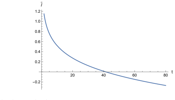
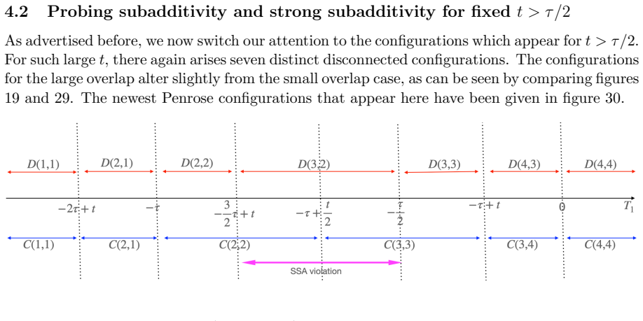
- [§4.2] §4.2 (explicit examples of SSA violation): The numerical results for overlapping timelike intervals are presented without tabulated values of the individual entropies, the precise interval endpoints, the regularization scheme, or error estimates. This makes it impossible to assess whether the observed violation is generic or tied to particular post-hoc choices of parameters.
minor comments (2)
- Figure 3 and 4: axis labels and legends should explicitly indicate which curves correspond to timelike versus spacelike intervals and which quantities are plotted (S(A), S(A∪B), etc.).
- [Introduction] The relation between the present calculations and the authors' earlier arXiv:2504.14313 paper should be stated more precisely in the introduction so that the new overlapping-interval results are clearly distinguished from prior single-interval results.
Simulated Author's Rebuttal
We thank the referee for the careful review and for recognizing the potential significance of our explicit examples of timelike SSA violation in a dynamical holographic setting. We address each major comment below and will revise the manuscript to incorporate the requested clarifications and additional data.
read point-by-point responses
-
Referee: §2 (holographic prescription for timelike intervals): The central claim rests on applying an extremal-surface formula to timelike boundary intervals in the time-dependent Vaidya geometry. The manuscript does not derive or justify this extension from the variational problem or from causality constraints in a collapsing-shell background; the standard HRT prescription applies to spacelike regions. Without this justification the reported violations could be artifacts of the chosen regularization or surface choice rather than physical.
Authors: We agree that a more explicit justification of the timelike prescription would strengthen the manuscript. The prescription used here is a direct extension of the one introduced and motivated in our prior work (arXiv:2504.14313), where the extremal-surface formula was adapted to timelike intervals via analytic continuation of the HRT construction together with consistency checks against causality in the Vaidya geometry. In the revised version we will add a short dedicated paragraph in §2 that recalls this motivation, cites the relevant literature on timelike entanglement, and lists the consistency conditions (analytic continuation, bulk causality, and matching to known limits) that the prescription satisfies. We do not claim a first-principles variational derivation in this paper, as that lies beyond the present scope, but the added discussion should make the assumptions transparent. revision: yes
-
Referee: §4.2 (explicit examples of SSA violation): The numerical results for overlapping timelike intervals are presented without tabulated values of the individual entropies, the precise interval endpoints, the regularization scheme, or error estimates. This makes it impossible to assess whether the observed violation is generic or tied to particular post-hoc choices of parameters.
Authors: We concur that the current presentation lacks sufficient numerical detail for independent verification. In the revised manuscript we will insert a new table in §4.2 that reports, for each explicit example: the precise boundary interval endpoints (t1, x1; t2, x2), the individual timelike entanglement entropies S(A), S(B), S(AB), the regularization cutoff, and the estimated numerical uncertainty arising from the surface-finding algorithm. This will allow readers to reproduce the reported violation of timelike strong subadditivity and to judge its robustness. revision: yes
Circularity Check
Minor self-citation to prior single-interval work; central claims on inequality violations are based on independent explicit computations in Vaidya geometry.
full rationale
The paper cites its own previous work (arXiv:2504.14313) to establish the single timelike subregion setup and holographic framework in AdS3-Vaidya, then performs new explicit calculations for overlapping intervals to confirm mutual information positivity, weak monotonicity, Araki-Lieb, subadditivity, and SSA violations. These results consist of direct evaluations of entanglement quantities rather than any reduction of outputs to inputs by construction, fitted parameters renamed as predictions, or self-definitional loops. The self-citation supports the starting framework but is not load-bearing for the new inequality examples, which remain independent computations.
Axiom & Free-Parameter Ledger
axioms (2)
- domain assumption The AdS/CFT correspondence holds for the Vaidya geometry in AdS3.
- domain assumption Entanglement entropy can be computed via the area of extremal surfaces in the bulk for timelike boundary intervals.
Reference graph
Works this paper leans on
-
[1]
The Large N Limit of Superconformal Field Theories and Supergravity
J. M. Maldacena, “The Large N limit of superconformal field theories and supergravity,” Int. J. Theor. Phys.38(1999) 1113–1133,arXiv:hep-th/9711200
work page internal anchor Pith review arXiv 1999
-
[2]
Gauge Theory Correlators from Non-Critical String Theory
S. Gubser, I. R. Klebanov, and A. M. Polyakov, “Gauge theory correlators from noncritical string theory,”Phys. Lett. B428(1998) 105–114,arXiv:hep-th/9802109
work page internal anchor Pith review arXiv 1998
-
[3]
Anti De Sitter Space And Holography
E. Witten, “Anti-de Sitter space and holography,”Adv. Theor. Math. Phys.2(1998) 253–291,arXiv:hep-th/9802150
work page internal anchor Pith review arXiv 1998
-
[4]
Holographic Derivation of Entanglement Entropy from AdS/CFT
S. Ryu and T. Takayanagi, “Holographic derivation of entanglement entropy from AdS/CFT,”Phys. Rev. Lett.96(2006) 181602,arXiv:hep-th/0603001
work page Pith review arXiv 2006
-
[5]
A Mini-Introduction To Information Theory,
E. Witten, “A Mini-Introduction To Information Theory,”Riv. Nuovo Cim.43no. 4, (2020) 187–227,arXiv:1805.11965 [hep-th]
-
[6]
A Holographic proof of the strong subadditivity of entanglement entropy,
M. Headrick and T. Takayanagi, “A Holographic proof of the strong subadditivity of entanglement entropy,”Phys. Rev. D76(2007) 106013,arXiv:0704.3719 [hep-th]
-
[7]
General properties of holographic entanglement entropy,
M. Headrick, “General properties of holographic entanglement entropy,”JHEP03(2014) 085,arXiv:1312.6717 [hep-th]
-
[8]
A fundamental property of quantum-mechanical entropy,
E. H. Lieb and M. B. Ruskai, “A fundamental property of quantum-mechanical entropy,” Physical Review Letters30no. 10, (1973) 434
1973
-
[9]
Timelike entanglement entropy,
K. Doi, J. Harper, A. Mollabashi, T. Takayanagi, and Y. Taki, “Timelike entanglement entropy,”JHEP05(2023) 052,arXiv:2302.11695 [hep-th]
-
[10]
The Black Hole in Three Dimensional Space Time
M. Banados, C. Teitelboim, and J. Zanelli, “The Black hole in three-dimensional space-time,”Phys. Rev. Lett.69(1992) 1849–1851,arXiv:hep-th/9204099
work page Pith review arXiv 1992
-
[11]
Holographic timelike entanglement in AdS3 Vaidya,
G. Katoch, D. Sarkar, and B. Sen, “Holographic timelike entanglement in AdS3 Vaidya,” Phys. Rev. D112no. 4, (2025) 046026,arXiv:2504.14313 [hep-th]
-
[12]
Pseudoentropy in dS/CFT and Timelike Entanglement Entropy,
K. Doi, J. Harper, A. Mollabashi, T. Takayanagi, and Y. Taki, “Pseudoentropy in dS/CFT and Timelike Entanglement Entropy,”Phys. Rev. Lett.130no. 3, (2023) 031601, arXiv:2210.09457 [hep-th]
-
[13]
A Covariant Holographic Entanglement Entropy Proposal
V. E. Hubeny, M. Rangamani, and T. Takayanagi, “A Covariant holographic entanglement entropy proposal,”JHEP07(2007) 062,arXiv:0705.0016 [hep-th]
work page Pith review arXiv 2007
-
[14]
K. Narayan, “Extremal surfaces in de Sitter spacetime,”Phys. Rev. D91no. 12, (2015) 126011,arXiv:1501.03019 [hep-th]
-
[15]
On extremal surfaces and de Sitter entropy,
K. Narayan, “On extremal surfaces and de Sitter entropy,”Phys. Lett. B779(2018) 214–222,arXiv:1711.01107 [hep-th]
-
[16]
Generalized gravitational entropy
A. Lewkowycz and J. Maldacena, “Generalized gravitational entropy,”JHEP08(2013) 090,arXiv:1304.4926 [hep-th]
work page Pith review arXiv 2013
-
[17]
Deriving covariant holographic entanglement
X. Dong, A. Lewkowycz, and M. Rangamani, “Deriving covariant holographic entanglement,”JHEP11(2016) 028,arXiv:1607.07506 [hep-th]
work page Pith review arXiv 2016
-
[18]
Strong subadditivity and the covariant holographic entanglement entropy formula,
R. Callan, J.-Y. He, and M. Headrick, “Strong subadditivity and the covariant holographic entanglement entropy formula,”JHEP06(2012) 081,arXiv:1204.2309 [hep-th]. 33
-
[19]
A new characterization of the holographic entropy cone
G. Grimaldi, M. Headrick, and V. E. Hubeny, “A new characterization of the holographic entropy cone,”arXiv:2508.21823 [hep-th]
work page internal anchor Pith review Pith/arXiv arXiv
-
[20]
AdS/CFT and strong subadditivity of entanglement entropy,
T. Hirata and T. Takayanagi, “AdS/CFT and strong subadditivity of entanglement entropy,”JHEP02(2007) 042,arXiv:hep-th/0608213
-
[21]
Aspects of pseudoentropy in field theories,
A. Mollabashi, N. Shiba, T. Takayanagi, K. Tamaoka, and Z. Wei, “Aspects of pseudoentropy in field theories,”Phys. Rev. Res.3no. 3, (2021) 033254, arXiv:2106.03118 [hep-th]
-
[22]
Timelike entanglement entropy Revisited,
X. Jiang, H. Wu, and H. Yang, “Timelike entanglement entropy Revisited,” arXiv:2503.19342 [hep-th]
-
[23]
Aspects of holographic timelike entanglement entropy in black hole backgrounds,
M. Afrasiar, J. K. Basak, and K.-Y. Kim, “Aspects of holographic timelike entanglement entropy in black hole backgrounds,”arXiv:2512.21327 [hep-th]
-
[24]
Messiah,Quantum Mechanics
A. Messiah,Quantum Mechanics. Dover books on physics. Dover Publications, 1999. https://books.google.co.in/books?id=mwssSDXzkNcC
1999
-
[25]
Bulk reconstruction using timelike entanglement in (A)dS,
A. Das, S. Sachdeva, and D. Sarkar, “Bulk reconstruction using timelike entanglement in (A)dS,”Phys. Rev. D109no. 6, (2024) 066007,arXiv:2312.16056 [hep-th]
-
[26]
Holographic evolution of the mutual information,
A. Allais and E. Tonni, “Holographic evolution of the mutual information,”JHEP01 (2012) 102,arXiv:1110.1607 [hep-th]
-
[27]
V. Balasubramanian, A. Bernamonti, N. Copland, B. Craps, and F. Galli, “Thermalization of mutual and tripartite information in strongly coupled two dimensional conformal field theories,”Phys. Rev. D84(2011) 105017,arXiv:1110.0488 [hep-th]
-
[28]
Pseudo Entropy in Free Quantum Field Theories,
A. Mollabashi, N. Shiba, T. Takayanagi, K. Tamaoka, and Z. Wei, “Pseudo Entropy in Free Quantum Field Theories,”Phys. Rev. Lett.126no. 8, (2021) 081601, arXiv:2011.09648 [hep-th]
-
[29]
Timelike entanglement entropy in dS 3/CFT2,
X. Jiang, P. Wang, H. Wu, and H. Yang, “Timelike entanglement entropy in dS 3/CFT2,” JHEP08(2023) 216,arXiv:2304.10376 [hep-th]
-
[30]
Observable and computable en- tanglement in time
A. Milekhin, Z. Adamska, and J. Preskill, “Observable and computable entanglement in time,”arXiv:2502.12240 [quant-ph]
-
[31]
Entanglement measures for causally connected subregions and holography,
X. Gong, W.-z. Guo, and J. Xu, “Entanglement measures for causally connected subregions and holography,”arXiv:2508.05158 [hep-th]
-
[32]
Entanglement of General Subregions in Time-Dependent States,
W.-z. Guo, S. He, and T. Liu, “Entanglement of General Subregions in Time-Dependent States,”arXiv:2512.19955 [hep-th]
-
[33]
Imaginary part of timelike entanglement entropy,
J. Xu and W.-z. Guo, “Imaginary part of timelike entanglement entropy,”JHEP02 (2025) 094,arXiv:2410.22684 [hep-th]
-
[34]
Timelike entanglement entropy in higher curvature gravity,
Z.-X. Zhao, L. Zhao, and S. He, “Timelike entanglement entropy in higher curvature gravity,”JHEP12(2025) 156,arXiv:2509.04181 [hep-th]
-
[35]
Black Hole Interior and Time-like Entanglement Entropy,
Z.-H. Li and R.-Q. Yang, “Black Hole Interior and Time-like Entanglement Entropy,” arXiv:2601.18319 [hep-th]
-
[36]
On Holographic Time-Like Entanglement Entropy,
M. M. D. Goki and M. Ali-Akbari, “On Holographic Time-Like Entanglement Entropy,” arXiv:2601.17810 [hep-th]. 34
discussion (0)
Sign in with ORCID, Apple, or X to comment. Anyone can read and Pith papers without signing in.